How to Actively Learn in Bounded Memory
A Brief Introduction: Enriched Queries and Memory Constraints
In the world of big-data, machine learning practice is dominated by massive supervised algorithms, techniques that require huge troves of labeled data to reach state of the art accuracy. While certainly successful in their own right, these methods break down in important scenarios like disease classification where labeling is expensive, and accuracy can be the difference between life and death. In a previous post, we discussed a new technique for tackling these high risk scenarios using enriched queries: informative questions beyond labels (e.g., comparing data points). While the resulting algorithms use very few labeled data points and never make errors, their efficiency comes at a cost: memory usage.
For simplicity, in this post we’ll consider the following basic setup. Let $X$ be a set of $n$ labeled points, where the labeling is chosen from some underlying family of classifiers (e.g., linear classifiers). As the learner, we are given access to the (unlabeled) points in $X$, a labeling oracle we can call to learn the label of any particular $x \in X$, and a set of special enriched oracles that give further information about the underlying classifier (e.g., a comparison oracle which can compare any two points $x,x’ \in X$). Our goal is to learn the label of every point in $X$ in as few queries (calls to the oracle) as possible.
Traditional techniques for solving this problem aim to use only $\log(n)$ adaptive queries. For instance if $X$ is a set of points on the real line and the labeling is promised to come from some threshold, we can achieve this using just a labeling oracle and binary search. This gives an exponential improvement over the naive algorithm of requesting the label of every point! However, these strategies generally have a problem: in order to choose the most informative queries, they allow the algorithm access to all of $X$, implicitly assuming the entire dataset is stored in memory. Since we frequently deal with massive datasets in practice, this strategy quickly becomes intractable. In this post, we’ll discuss a new compression-based characterization of when its possible to learn in $\log(n)$ queries, but store only a constant number of points in the process.
A Basic Example: Learning Thresholds via Compression
Learning in constant memory may seem a tall order when the algorithm is already required to correctly recover every label in a size $n$ set $X$ in only $\log(n)$ queries. To convince the reader such a feat is even possible, let’s start with a fundamental example using only label queries: thresholds in 1D. Let $X$ be any set of $n$ points on $\mathbb{R}$ with (hidden) labels given by some threshold. We’d like to learn the label of every point in $X$ in around $\log(n)$ adaptive queries of the form “what is the label of $x \in X$?” Notice that to do this, it is enough to find the points directly to the right and left of the threshold—the only issue is we don’t know where they are! Classically, we’d try find these points using binary search. This would acheive the $\log(n)$ bound on queries, but determining which point to query in each step requires too much memory.
A better strategy for this problem was proposed by Kane, Lovett, Moran, and Zhang (KLMZ). They follow a simple four step process:
- Randomly sample $O(1)$ points from remaining set (initially $X$ itself).
- Query the labels of these points, and store them in memory.
- Restrict to the set of points whose labels remain unknown.
- Repeat $O(\log(n))$ times.
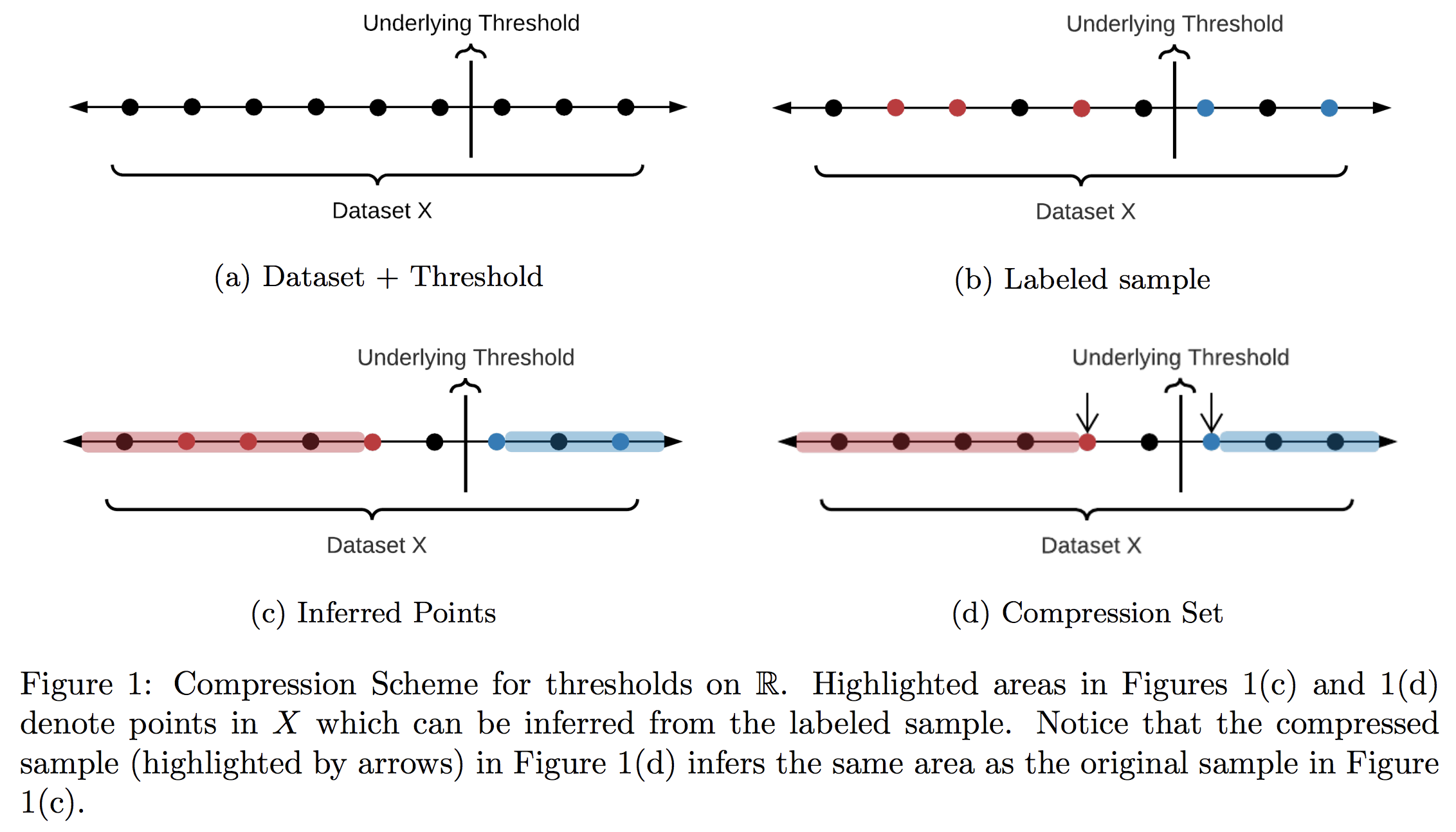
Note that it is possible to remove points we have not queried in Step 3 (we call such points “inferred,” see Figure 1(c)). Indeed, KLMZ prove that despite only making $O(1)$ queries, each round should remove about half of the remaining points. As a result, after about $\log(n)$ rounds, we must have found the two points on either side of the threshold, and can therefore label all of $X$ as desired (see our previous post for more details on this algorithm). This algorithm is much better than binary search, but it still stores $O(\log(n))$ points overall—we’d like an algorithm whose memory doesn’t scale with $n$ at all!
It turns out that for the class of thresholds, this can be achieved by a very simple tactic: in each round, only store the two points closest to each side of the threshold. This “compressed” version of the sample actually retains all relevant information, so the algorithm’s learning guarantees are completely unaffected. Let’s take a look pictorially.
Since we can compress our storage down to a constant size in every round and never draw more than $O(1)$ points, this strategy results in a learner whose memory has no dependence on $X$ at all: a zero-error, query efficient, bounded memory learner.
A General Framework: Lossless Sample Compression
Our example for thresholds in 1D suggests the following paradigm: if we can compress samples down to $O(1)$ points without harming inference, bounded memory learning is possible. This is true, but not particularly useful: most classes beyond thresholds can’t even be actively learned (e.g., halfspaces in $2D$), much less in bounded memory. To build learners for classes beyond thresholds, we’ll need to generalize our idea of compression to the enriched query regime. In more detail, let $X$ be a set and $H$ a family of binary labelings of $X$. We consider classes $(X,H)$ with an additional query set $Q$. Formally, $Q$ consists of a set of oracles that contain information about the set $X$ based upon the structure of the underlying hypothesis $h \in H$. Our formal definition of these oracles is fairly broad (see our paper for exact details), but they can be thought of simply as functions dependent on the underlying hypothesis $h \in H$ that give additional structural information about tuples in $X$. One standard example is the comparison oracle on halfspaces. Given a particular halfspace $\langle \cdot, v \rangle$, the learner may send a pair $x,x’$ to the comparison oracle to learn which example is closer to the decision boundary, or equivalently they recieve $\text{sign}(\langle x, v \rangle - \langle x’, v \rangle)$).
To generalize our compression-based strategy for thresholds to the enriched query setting, we also need to discuss a little bit of background on the theory of inference. Let $(X,H)$ be a hypothesis class with associated query set $Q$. Given a sample $S \subset X$ and query response $Q(S)$, denote by $H_{Q(S)}$ the set of hypotheses consistent with $Q(S)$ (also called the version space, this is the set of $h \in H$ such that $Q(S)$ is a valid response if $h$ is the true underlying classifier). We say that $Q(S)$ infers some $x \in X$ if all consistent classifiers label $x$ the same, that is if there exists $z \in$ {$0,1$} such that: \[ \forall h \in H_{Q(S)}, h(x)=z. \] This allows us to label $x$ with 100% certainty, since the true underlying classifier must lie in $H_{Q(S)}$ by definition, and all such classifiers give the same label to $x$!
In the case of thresholds, our compression strategy relied on the fact that the two points closest to the boundary inferred the same amount of information as the original sample. We can extend this idea naturally to the enriched query regime as well.
Recall our goal is to correctly label every point in $X$. Using lossless compression, we can now state our general algorithm for this process:
- Randomly sample $O(1)$ points from remaining set (initially $X$ itself).
- Make all queries on these points, and store them in memory.
- Compress memory via the lossless compression scheme.
- Restrict to the set of points whose labels remain unknown.
- Repeat $O(\log(n))$ times.
In recent work with Daniel Kane, Shachar Lovett, and Michal Moshkovitz, we prove that this basic algorithm achieves zero-error, query optimal, bounded memory learning.
\[ O_k(\log(n)) \text{ queries} \] and \[ O_k(1) \text{ memory}. \]
Before moving on to some examples, let’s take a brief moment to discuss the proof. The result essentially follows in two steps. First, we’d like to show that for any distribution over $X$, drawing $O(k)$ points is sufficient to infer $1/2$ of $X$ in expectation. This follows similarly to standard results in the literature—one can either use the classic sample compression arguments of Floyd and Warmuth, or more recent symmetry arguments of KLMZ. With this in hand, it’s easy to see that after $\log(n)$ rounds (learning $1/2$ of $X$ each round), we’ll have learned all of $X$. The second step is then to observe that our compression in each step has no effect on this learning procedure. This follows without too much difficulty from the definition of lossless sample compression, which promises that the compressed sub-sample preserves all such information.
Example: Axis-Aligned Rectangles
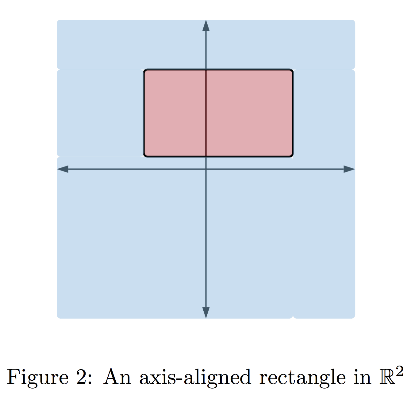
While interesting in its own right, a sufficient condition like Lossless Sample Compression is most useful if it applies to natural classifiers. We’ll finish our post by discussing an application of this paradigm to labeling a dataset $X$ when the underlying classifier is given by an axis-aligned rectangle. Axis-aligned Rectangles are a natural generalization of intervals to higher dimensions. They are given by a product of $d$ intervals in $\mathbb{R}$: \[ R = \prod\limits_{i=1}^d [a_i,b_i], \] such that an example $x=(x_1,\ldots,x_d) \in \mathbb{R}^d$ lies in the rectangle if every feature lies inside the specified interval, that is $x_i \in [a_i,b_i]$.
Standard arguments show that with only labels, learning the labels of a set $X$ of size $n$ takes $\Omega(n)$ queries in the worst case when the labeling is given by some underlying rectangle. To see why, let’s consider the simple case of 1D—intervals. The key observation is that a sample of points $S_{\text{out}}$ lying outside the interval cannot infer any information beyond its own labels. This is because for any $x \in \mathbb{R} \setminus S_{\text{out}}$, there exists an interval that includes $x$ but not $S_{\text{out}}$ (say $I=[x-\varepsilon,x+\varepsilon]$ for some small enough $\varepsilon$), and an interval that excludes $x$ and $S_{\text{out}}$ (say $I=[x+\varepsilon,x+2\varepsilon]$). As a result, we cannot tell whether $x$ is included in the underlying interval. In turn, this means that if we try to compress $S_{\text{out}}$ in any way, we will always lose information about the original sample.
To circumvent this issue, we introduce “odd-one-out” queries. This new query type allows the learner to take any point $x\in X$ in the dataset that lies outside of the rectangle $R$, and ask for a violated coordinate (i.e. a feature lying outside one of the specified intervals) and the direction of violation (was the coordinate too large, or too small?). Concretely, imagine a chef is trying to cook a dish for a particularly picky patron. After each failed attempt, the chef asks the patron what went wrong, and the patron responds with some feature they dislike (perhaps the meat was overcooked, or undersalted). It turns out that such scenarios have small lossless compression schemes (and are therefore learnable in bounded memory).
We’ll wrap up our post by sketching the proof. It will be convenient to break our compression scheme into two parts: a scheme for points inside the rectangle, and a scheme points outside the rectangle.1
Let’s start with the former case and restrict our attention to a sample of points $S_{\text{in}}$ that lies entirely inside the rectangle. We claim that all the relevant information in this case is captured by the maximum and minimum values of coordinates in $S_{\text{in}}$. Storing the $2d$ points achieving these values can be viewed as storing a bounding box that is guaranteed to lie inside the underlying rectangle classifier.
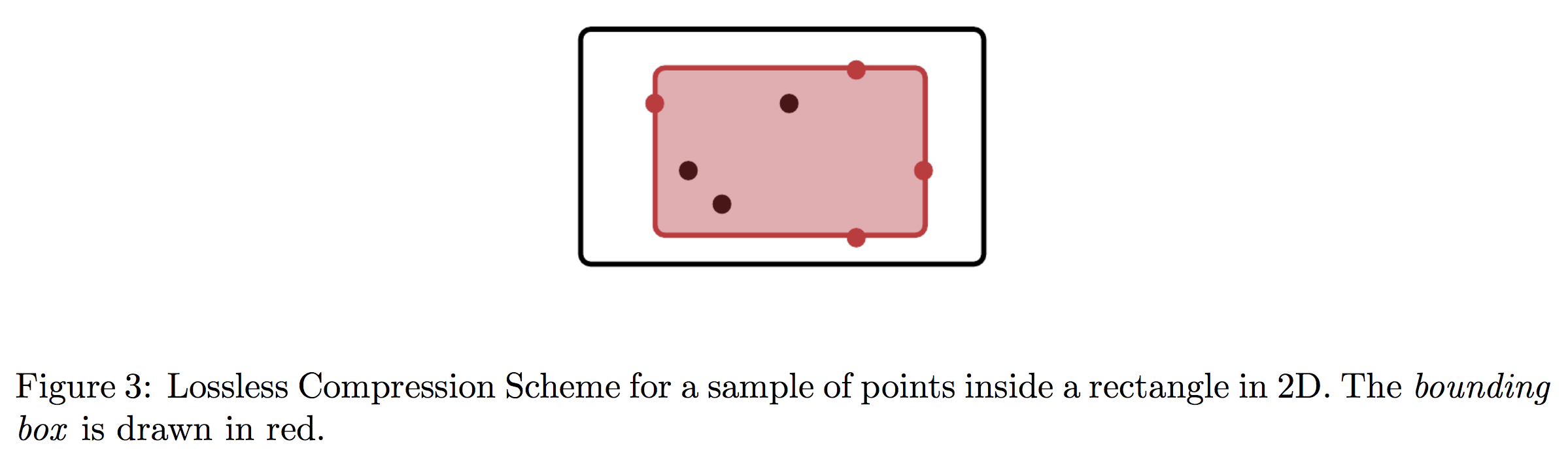
Notice that for any point $x \in \mathbb{R}^d$ outside of the bounding box, the version space (that is the set of all rectangles that contain $S_{\text{in}}$) has both a rectangle that contains $x$, and a rectangle that does not contain $x$. This means that label queries on $S_{\text{in}}$ cannot infer any point outside of the bounding box. Since every point inside the box is inferred by the compressed sample, these $2d$ points give a compression set for $S_{\text{in}}$.
Now let’s restrict our attention to a sample $S_{\text{out}}$ that lies entirely outside the rectangle. In this case, we’ll additionally have to compress information given by the odd-one-out oracle as well as labels. Nevertheless, we claim that a simple strategy suffices: store the closest point to each edge of the rectangle.
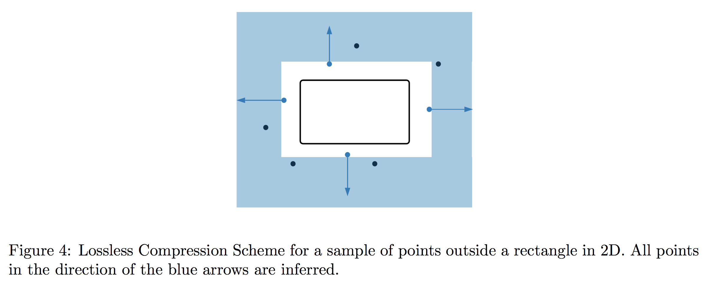
In particular, because the odd-one-out oracle gives a violated coordinate and direction of violation, any point that is further out in the direction of violation must also lie outside the rectangle. In any given direction, it is not hard to see that all relevant information is captured by the closest point to the relevant edge, since any further point can be inferred to be too far in that direction.
Conclusion
We’ve now seen that lossless sample compression, the ability to compress finite samples without loss of label inference, gives a simple algorithm for labeling an $n$-point dataset $X$ in $O(\log(n))$ queries while never storing more than $O(1)$ examples at a time. Furthermore, we’ve shown that lossless compression isn’t a hopelessly strong condition—basic real-world questions such as the odd-one-out query often lead to small compression schemes. In our recent paper we give a few more examples of this phenomenon for richer classes such as decision trees and halfspaces in 2D.
On the other hand, there is still much left to explore! Lossless sample compression gives a sufficient condition for bounded memory active learning, but it is not clear if the condition is necessary. The parameter is closely related to a necessary condition for active learning called inference dimension (see our previous post or KLMZ’s original paper for a description), and it is an open problem whether these two measures are equivalent. A positive resolution would imply that every actively learnable class is also actively learnable in bounded memory! Finally, it is worth noting that the techniques we discuss in this post are not robust to noise. Building a general framework for the more realistic noise-tolerant regime remains an interesting open question as well.
Footnotes
-
Note that this does not immediately imply a compression set for general samples. However, the definition of lossless compression can be weakened to allow for seperate compression schemes for positive and negative examples without affecting the resulting implications on bounded memory learnability. ↩