The Power of Comparison: Reliable Active Learning
With the surge of widely available massive online datasets, we have become very good at building algorithms which distinguish between the following:
But what about solving classification problems which may have large unlabeled datasets, but whose labeling requires expert advice? What about situations like examining an MRI scan or recognizing a pedestrian, where a mistake in classification could be the difference between life and death? In these situations, it would be great if we could build a classification algorithm with the following properties:
- The algorithm requires very few labeled data points to train.
- The algorithm never makes a mistake.
This raises an obvious question: is building an efficient algorithm with such strong guarantees even possible? It turns out the answer is yes—just not in the standard learning model. In recent joint work with Daniel Kane and Shachar Lovett, we show that while it is impossible to have such guarantees using only the labels of data points, achieving the goal becomes easy if you give the algorithm a little more power.
Comparison Queries
Our work explores the additional power of algorithms which are allowed to compare data. In slightly more detail, imagine points in $\mathbb{R}^d$ are labeled by a linear classifier: that is $\text{sign}(f)$ for some affine linear function $f(x) = \langle x, w \rangle + b$.
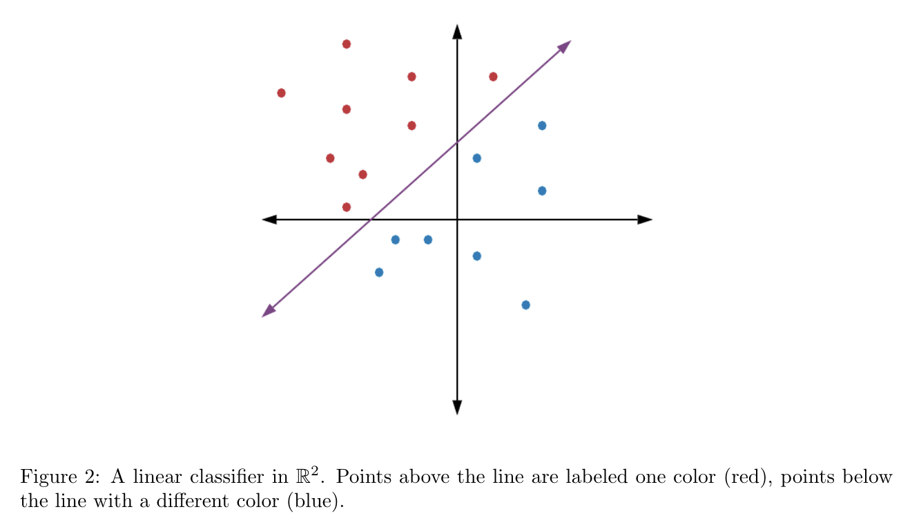
A comparison between two data points $x,y \in \mathbb{R}^d$ asks which point is closer to the decision boundary (e.g. the purple line in Figure 2). More formally, a comparison query asks: \[ f(x) - f(y) \overset{?}{\geq} 0. \] On the other hand, a standard label query on $x \in \mathbb{R}^d$ only asks which side of the decision boundary $x$ lies on, i.e. \[ f(x) \overset{?}{\geq} 0. \] Comparison queries are natural from a human perspective—think how often throughout your day you compare objects, ideas, or alternatives. In fact, it has even been shown that in many practical circumstances, we may be better at accurately comparing objects than we are at labeling them! Since we are allowing our algorithm access to an expert (possibly human) oracle, it makes sense to allow the algorithm to ask the expert to compare data.
The Algorithm
How can we use comparisons to learn with few queries and no mistakes? It turns out that a remarkably simple algorithm suffices! Imagine you are given a finite sample $S \subset \mathbb{R}^d$, and would like to find the label of every point in $S$ without making any errors. Consider the following basic procedure:
- Draw a small subsample $S’ \subset S$
- Send $S’$ to the oracle to learn both labels and comparisons
- Remove points from $S$ whose labels are learned in Step 2, and repeat.
How exactly does Step 2 “learn labels”? Formally, this is done through a linear program whose constraints are given by the oracle responses on $S’$. Informally, this has a nice geometric interpretation. Let’s consider first the two dimensional case, originally studied by Kane, Lovett, Moran, and Zhang (KLMZ). Figure 3 shows how comparisons allow us to infer the labels of points in $S$ by building cones (one red, one blue) based on the query results on $S’$. In essence, comparison queries allow us to find the points in $S’$ closest to the decision boundary (Figure 3(c)), which we call minimal. By drawing a cone stemming from a minimal point to others of the same label (Figure 3(d)), we can infer that every point inside the cone must share the same label as well (Figure 3(e)).
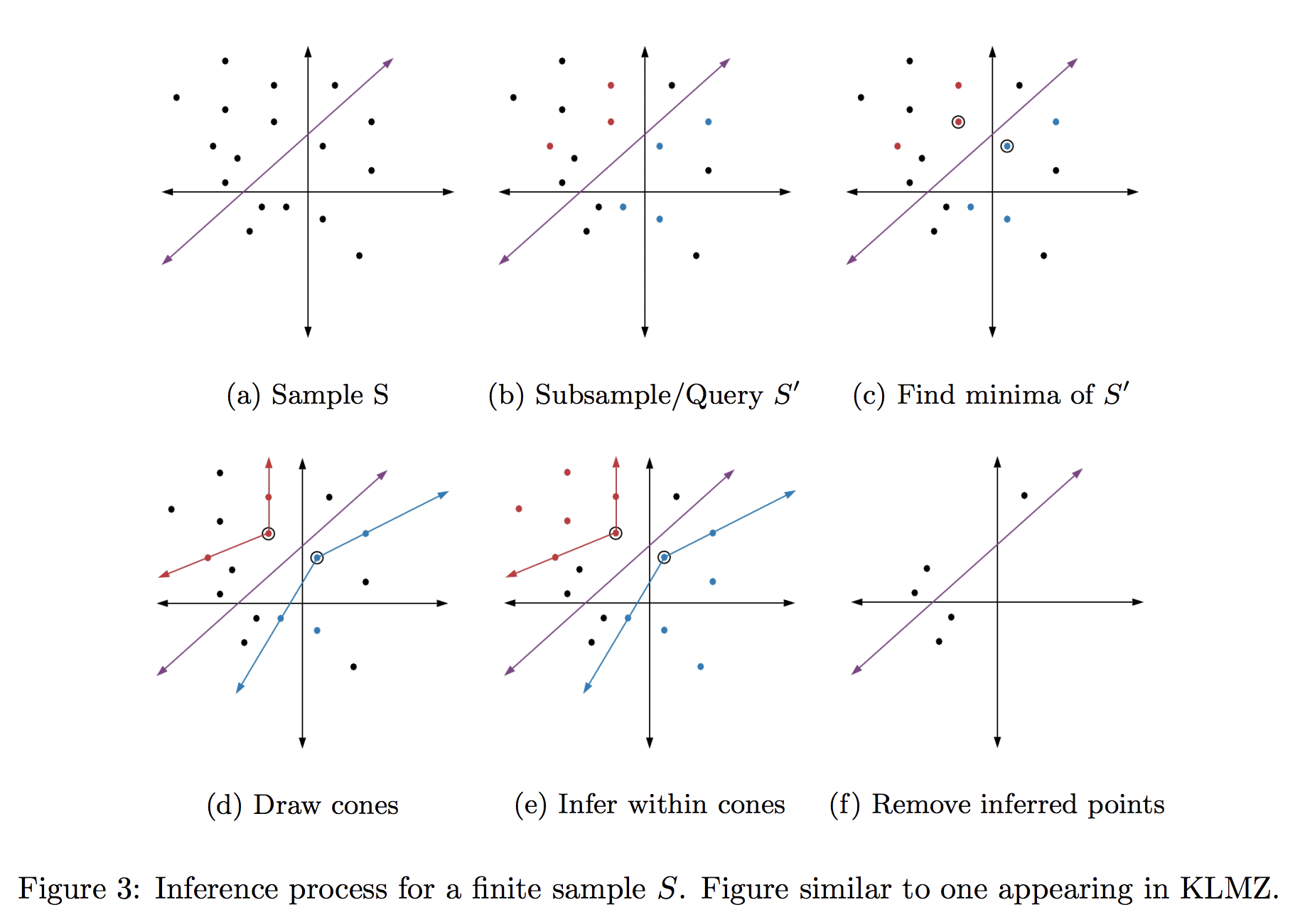
Why does this process satisfy our guarantees? Let’s first discuss why we never mislabel a point, which follows from the fact that our cones stem from minima. Because our classifier is linear, this guarantees that the edges of our cones do not cross the decision boundary (i.e. change labels). Thus, the label of any point inside such a cone must be the same as its base point! Notice that this only remains true so long as the base point of our cone is minimal, which explains why comparison queries, the mechanism through which we find minima, are crucial to the algorithm.
The second guarantee, ensuring that we make few queries overall, is a bit more subtle, and requires the combinatorial theory of inference dimension.
Inference and Average Inference Dimension
Inference dimension is a complexity parameter introduced by KLMZ to measure how large a subsample $S’$ must be in order to learn a constant fraction of $S$.
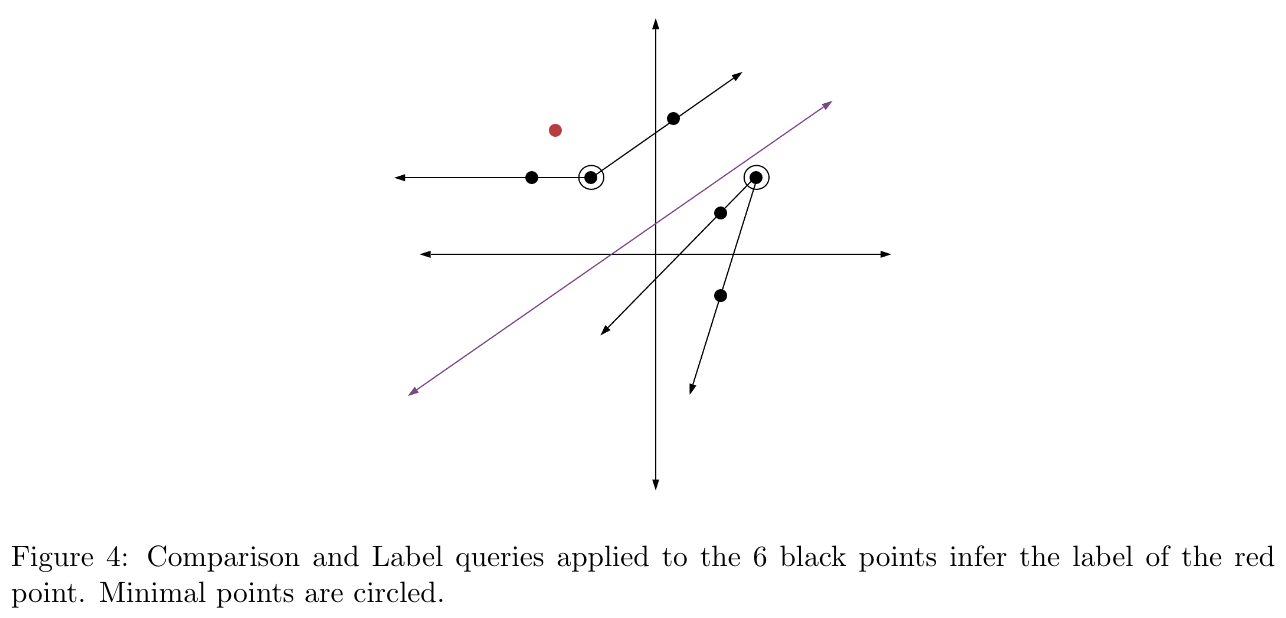
Let’s take a look at an example, linear classifiers in two dimensions. Figure 4 shows that this class has inference dimension at most 7. Why? A sample of size 7 will always have at least 4 points with the same label, and the label of one of these points can always be inferred from labels and comparisons on the rest!
KLMZ show that by picking the size of $S’$ to be just a constant times larger than the inference dimension, the resulting cones will usually cover a constant fraction of our distribution. In other words, in two dimensions, every round of our algorithm infers a constant fraction of the remaining points, which means we only need $O(\log(|S|))$ rounds before our algorithm has labeled everything!
Unfortunately, in 3+ dimensions, linear classifiers become harder to deal with—indeed KLMZ show that their inference dimension is infinite. In our recent work, we circumvent this issue by applying a standard assumption from the data science and learning literature: we assume that our sample $S$ is drawn from some restricted range of natural distributions. The core idea of our analysis is then based off of a simple lemma, which informally states that even if $(X,H)$ has infinite inference dimension, samples from $X$ may still have small inference dimension with high probability!
\[ \Pr[\text{Inference dimension of} \ (S,H) \leq k] \geq 1-{ n \choose k}g(k). \]
The main technical difficulty then becomes showing that $g(k)$, which we term average inference dimension, is indeed small over natural distributions. We confirm that this is the case for the class of s-concave distributions $(s \geq -\frac{1}{2d+3})$, a wide ranging generalization of Gaussians that includes fatter-tailed distributions like the Pareto and t-distribution.
\[ g(k) \leq 2^{-\tilde{\Omega}\left(\frac{k^2}{d}\right)}. \]
Plugging this into our observation, we see that as long as $S$ is reasonably large, it will have inference dimension $\tilde{O}(d\log(|S|))$ with high probability! This allows us to efficiently learn the labels of $S$ through the algorithm we discussed before, so long as the distribution is s-concave. As a corollary, we get the following result:
\[ \tilde{O}(d\log(|S|)^2) \] expected queries, as long as $S$ is drawn from an s-concave distribution.
While we have focused in the above on learning finite samples, it turns out satisfying similar guarantees over all of $\mathbb{R}^d$ (under natural distributions) is also possible via the same argument. In this case, rather than trying to learn the label of every point, we allow our algorithm to respond “I don’t know” on an $\varepsilon$ fraction of samples. This type of algorithm goes by many names in the literature, perhaps the catchiest of which is a “Knows What It Knows” (KWIK) learner. The above then (with a bit of work) more or less translates into a KWIK-learner1 that uses only $d\log(1/\varepsilon)^2$ calls to the oracle.
Lower Bound
Why doesn’t this algorithm work with only labels? It’s long been known that even in two dimensions, achieving these learning guarantees is impossible for certain adversarial distributions such as $S^1$. Let’s take a look at how our results match up on a less adversarial example with a long history in learning theory: the d-dimensional unit ball.
\[ \tilde{O}(d\log^2(1/\varepsilon)) \] oracle calls. On the other hand, using only labels takes at least \[ \left (\frac{1}{\varepsilon}\right)^{\Omega(d)} \] oracle calls2.
This simple example shows the exponential power of comparisons: moving KWIK-learning from intractable to highly efficient. As a final note, implementing the algorithm amounts to running a series of small linear programs, and as a result is computationally efficient as well, only taking about $\text{poly}\left(\frac{1}{\varepsilon},d\right)$ time.
It remains to be seen whether this type of efficient, comparison-based KWIK-learning will be useful in practice. Comparison queries have already been shown to provide practical improvements over labels for similar learning problems, and have been used to great effect in other areas such as recommender systems, search, and ranking as well. Since we have recently extended our results to more realistic noisy scenarios in joint work with Gaurav Mahajan, we are optimistic that our techniques will remain as powerful in practice as they are in theory.
Footnotes
-
It’s worth noting that we have abused notation here. Formally, our algorithms do not fall into the KWIK-model, but are built in a similar learning-theoretic framework called RPU-learning. ↩
-
This follows from a standard cap packing argument—we can divide up the ball into many disjoint caps, and note that any KWIK-learner must query a point in at least half of them to be successful. ↩