Explainable 2-means Clustering: Five Lines Proof
TL;DR: we will show why only one feature is enough to define a good $2$-means clustering. And we will do it using only 5 inequalities (!) In a previous post, we explained what is an explainable clustering.
Explainable clustering
In a previous post, we discussed why explainability is important, defined it as a small decision tree, and suggested an algorithm to find such a clustering. But why the resulting clustering is any good?? We measure “good” by $k$-means cost. The cost of a clustering $C$ is defined as the sum of squared Euclidean distances of each point $x$ to its center $c(x)$. Formally, \begin{equation} cost(C)=\sum_x \|x-c(x)\|^2, \end{equation} the sum is over all points $x$ in the dataset.
In this post, we focus on the $2$-means problem, where there are only two clusters. We want to show that for every dataset there is one feature $i$ and one threshold $\theta$ such that the following simple clustering $C^{i,\theta}=(C^{i,\theta}_1,C^{i,\theta}_2)$ has a low cost: \begin{equation} \text{if } x_i\leq\theta \text{ then } x\in C^{i,\theta}_1 \text{ else } x\in C^{i,\theta}_2. \end{equation} We call such a clustering a threshold cut. There might be many threshold cuts that are good, bad, or somewhere in between. We want to show that there is at least one that is good (i.e., low cost). In the paper, we prove that there is always a threshold cut, $C^{i,\theta}$, that is almost as good as the optimal clustering: \begin{equation} cost(C^{i,\theta})\leq4\cdot cost(opt), \end{equation} where $cost(opt)$ is the cost of the optimal 2-means clustering. This means that there is a simple explainable clustering $C^{i,\theta}$ that is only $4$ times worse than the optimal one. It’s independent of the dimension and the number of points. Sounds crazy, right? Let’s see how we can prove it!
The minimal-mistakes threshold cut
We want to compare two clusterings: the optimal clustering and the best threshold cut. The best threshold cut is hard to analyze, so we introduce an intermediate clustering: the minimal-mistakes threshold cut, $\widehat{C}$. Even though this clustering will not be the best threshold cut, it will be good enough. In the paper we prove that $cost(\widehat{C})$ is at most $4cost(opt)$. For simplicity, in this post, we will show a slightly worse bound of $11cost(opt)$ instead of $4cost(opt)$.
We define the number of mistakes of a threshold cut $C^{i,\theta}$ as the number of points $x$ that are not in the same cluster as their optimal center $c(x)$ in $C^{i,\theta}$, i.e., number of points $x$ such that
\begin{equation}
sign(\theta-x_i) \neq sign(\theta-c(x)_i).
\end{equation}
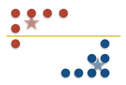
The minimal-mistakes clustering is the threshold cut that has the minimal number of mistakes. Take a look at the next figure for an example.
Playing with cost: warm-up
Before we present the proof, let’s familiarize ourselves with the $k$-means cost and explore several of its properties. It will be helpful later on!
Changing centers
If we change the centers of a clustering from their means (which are their optimal centers) to different centers $c=(c_1, c_2)$, then the cost can only increase. Putting this into math, denote by $cost(C,c)$ the cost of clustering $C=(C_1,C_2)$ when $c_1$ is the center of cluster $C_1$ and $c_2$ is the center of cluster $C_2$, then
\begin{align} cost(C) &= \sum_{x\in C_1} \|x-mean(C_1)\|^2 + \sum_{x\in C_2} \|x-mean(C_2)\|^2 \newline &\leq \sum_{x\in C_1} \|x-c_1\|^2 + \sum_{x\in C_2} \|x-c_2\|^2 = cost(C,c). \end{align} What if we further want to change the centers from some arbitrary centers $(c_1, c_2)$ to other arbitrary centers $(m_1, m_2)$? How does the cost change? Can we bound it? To our rescue comes the (almost) triangle inequality that states that for any two vectors $x,y$: \begin{equation} \|x+y\|^2 \leq 2\|x\|^2+2\|y\|^2. \end{equation} This implies that the cost of changing the centers from $c=(c_1, c_2)$ to $m=(m_1, m_2)$ is bounded by \begin{equation} cost(C,c)\leq 2cost(C,m)+2|C_1|\|c_1-m_1\|^2+2|C_2|\|c_2-m_2\|^2. \end{equation}
Decomposing the cost
The cost can be easily decomposed with respect to the data points and the features. Let’s start with the data points. For any partition of the points in $C$ to $S_1$ and $S_2$, the cost can be rewritten as \begin{equation} cost(C,c)=cost(C \cap S_1,c)+cost(C \cap S_2,c). \end{equation} The cost can also be decomposed with respect to the features, because we are using the squared Euclidean distance. To be more specific, the cost incur by the $i$-th feature is $cost_i(C,c)=\sum_{x}(x_i-c(x)_i)^2,$ and the total cost is equal to \begin{equation} cost(C,c)=\sum_i cost_i(C,c). \end{equation} If the last equation is unclear just recall the definition of the cost ($c(x$) is the center of a point $x$): \begin{equation} cost(C,c)=\sum_{x}\|x-c(x)\|^2=\sum_i\sum_{x}(x_i-c(x)_i)^2=\sum_icost_i(C,c). \end{equation}
The 5-line proof
Now we are ready to prove that $\widehat{C}$ is only a constant factor worse than the optimal $2$-means clustering: \begin{equation} cost(\widehat{C})\leq 11\cdot cost(opt). \end{equation}
To prove that the minimal-mistakes threshold cut $\widehat{C}$ gives a low-cost clustering, we will do something that might look strange at first. We analyze the quality of this clustering $\widehat{C}$ with the optimal centers of the optimal clustering. And not the optimal centers for $\widehat{C}$. This step will only increase the cost, so why are we doing it — because it will ease our analysis, and if there are not many mistakes, then the centers do not change much, like in the previous figure. So it’s not much of an increase. So, here comes the first step — change the centers of $\widehat{C}$ to the optimal centers $c^*=(mean(C^*_1),mean(C^*_2))$. Recall from the warm-up that this can only increase the cost: \begin{equation} cost(\widehat{C})\leq cost(\widehat{C},c^{*}) \quad (1) \end{equation} Next we use one of the decomposition properties of the cost. We partition the dataset into the set of points that are correctly labeled, $X^{cor}$, and those that are not, $X^{wro}$.
Thus, we can rewrite the last term as \begin{equation} cost(\widehat{C},c^{*})=cost(\widehat{C}\cap X^{cor},c^{*})+cost(\widehat{C}\cap X^{wro},c^{*}) \quad (2) \end{equation}
Let’s look at this sum. The first term contains all the points that have their correct center in $c^*$ (which is either $mean(C^*_1)$ or $mean(C^*_2)$). Hence, the first term in (2) is easy to bound: it’s at most $cost(opt)$. So from now on, we focus on the second term.
In the second term, all points are in $X^{wro}$, which means they were assigned to the incorrect optimal center. So let’s change the centers once more, so that $X^{wro}$ will have the correct centers. The correct centers of $X^{wro}$ are the same centers $c^*$, but the order is reversed, i.e., all points assigned to center $mean(C^*_1)$ are now assigned to $mean(C^*_2)$ and vice versa. Using the “changing centers” property of the cost we discussed earlier, we have
\begin{equation} cost(\widehat{C},c^{*}) \leq 3cost(opt)+2|X^{wro}|\cdot\|c^{*}_1-c^{*}_2\|^2 \quad (3) \end{equation}
Now we’ve reached the main step in the proof. We show that the second term in (3) is bounded by $8cost(opt)$. We first decompose $cost(opt)$ using the features. Then, all we need to show is that:
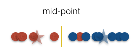
\begin{equation} cost_i(opt)\geq\left(\frac{|c^{*}_{1,i}-c^{*}_{2,i}|}{2}\right)^2|X^{wro}| \quad (4) \end{equation}
The trick is, for each feature, to focus on the threshold cut defined by the middle point between the two optimal centers. Since $\widehat{C}$ is the minimal-mistakes clustering we know that in every threshold cut there are at least $|X^{wro}|$ mistakes. Each mistake contributes at least half the distance between the two centers.
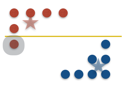
This figure shows how to prove step (4). We see that there is $1$ mistake, which is the minimum possible. This means that even the optimal clustering must pay for at least half the distance between the centers for each of these mistakes. This gives us a lower bound on $cost_i(opt)$ in this feature. Then we can sum over all the features to see that the second term of (3) is at most $8cost(opt)$, which is what we wanted. Putting everything together, we get exactly what we wanted to prove in this post: \begin{equation} cost(\widehat{C})\leq1 1\cdot cost(opt) \quad (5) \end{equation}
Epilogue: improvements
The bound that we got, $11$, is not the best possible. With more tricks we can get a bound of $4$. One of them is using Hall’s theorem. Similar ideas provide a $2$-approximation to the optimal $2$-medians clustering as well. To complement our upper bounds, we also prove lower bounds showing that any threshold cut must incur almost $3$-approximation for $2$-means and almost $2$-approximation for $2$-medians. You can read all about it in our paper.