Understanding Instance-based Interpretability of Variational Auto-Encoders
Background: Instance-based Interpretability
Modern machine learning algorithms can achieve very high accuracy on many tasks such as image classification. Despite their great success, these algorithms are often black boxes as their predictions are mysterious to humans. For example, when we feed an image to a dog-versus-cat classifier, it says: “After a matrix product and max pooling and a non-linearity and a skip connection and another 100 math operations, look, the probability that ‘this image is a cat’ is 99%!” Unfortunately, this makes no sense to a human at all. To understand what is going on, we need information that can be easily interpreted by human. One way to provide more interpretable answer is to ask:
This is called a counterfactual question. Instance-based interpretation methods answer this question by designing an interpretability score between every training sample and the test sample. High scores imply importance. Then, we can interpret the prediction by saying: the classifier labels the test image as a cat because these other training samples are cats, and they are most responsible for the prediction of the test image.
The notion of influence functions is a popular instance-based interpretability method for supervised learning. The intuition is: if removing some $x$ in the training set results in a large difference of the prediction (such as the logits) of $z$, then $x$ is very important for the prediction of $z$. Imagine $z$ is a very special cat that is visually different from all training images except for one sample $x$. Then, $x$ has large influence over $z$ because removing $x$ probably leads to an incorrect prediction of $z$.
Interpretations for Unsupervised Learning
For supervised learning, instance-based interpretability methods reveal why a classifier makes a certain prediction. What about unsupervised learning? Our recent paper investigates this problem for several unsupervised learning methods. The first challenge is, how do we frame the counterfactual question in unsupervised learning?
When the model fits a probability density to the training data, we ask: which training samples are most responsible for increasing the log-likelihood of a test sample? In deep generative models such as variational auto-encoders (VAE), likelihood is not available. VAEs are optimized to maximize the evidence lower bound (ELBO) of the log-likelihood. Then, we ask: which training samples are most responsible for increasing the ELBO of a test sample?
Then, these questions can readily be answered by influence functions with proper loss functions. Formally, let $X=\{x_1,\cdots,x_n\}$ be the training set, and $\mathcal{A}$ be the unsupervised model. That is, $\mathcal{A}(X)$ returns the model fit to $X$. Let $L(X;\mathcal{A}) = \frac1N \sum_{i=1}^N \ell(x_i;\mathcal{A}(X))$ be the loss function, where the loss $\ell$ is negative log-likelihood in density estimators and negative ELBO in VAE. Then, the influence function of a training sample $x_i$ over a test sample $z$ is the difference of the losses at $z$ between models trained with and without $x_i$. Formally, we define the influence function as \[\mathrm{IF}_{X,\mathcal{A}}(x_i,z) = \ell(z;\mathcal{A}(X\setminus\{x_i\})) - \ell(z;\mathcal{A}(X)).\] We provide intuition for influence functions in the next section.
What Should Influence Functions Tell Us?
What does it mean if $\mathrm{IF}(x_i,z)\gg0$? Straightforward, we have $\ell(z;\mathcal{A}(X\setminus\{x_i\})) \gg \ell(z;\mathcal{A}(X))$, which means removing $x_i$ should result in a large increase of the loss at $z$. In other words, $x_i$ is very important for the model $\mathcal{A}$ to learn $z$. Similarly, if $\mathrm{IF}(x_i,z)\ll0$, then $x_i$ negatively impacts the model in learning $z$; and if $\mathrm{IF}(x_i,z)\approx0$, then $x_i$ hardly impacts it.
For conciseness, we call training samples that have positive / negative influences over a test sample $z$ proponents / opponents of $z$. In supervised learning, strong proponents and opponents of $z$ are very important to explain the model’s prediction of $z$. Strong proponents help the model correctly predict the label of $z$ because they reduce the loss at $z$, while strong opponents harm it because they increase the loss at $z$. Empirically, strong proponents of $z$ are visually its similar samples from the same class, while strong opponents of $z$ are usually its dissimilar samples from the same class or its similar samples from a different class.
In unsupervised learning, we expect that strong proponents increase the likelihood of $z$ and strong opponents reduce it, so we ask:
In particular, when we let $z = x_i$, we obtain a concept called self influence, or $\mathrm{IF}(x_i,x_i)$. This concept is very interesting in supervised learning because self influences provide rich information about memorization of training samples. For example, Feldman and Zhang study neural network memorization through the lens of self influences in this paper. Intuitively, high self influence samples are atypical, ambiguous or mislabeled, while low self influence samples are typical. We want to know what self influences reveal in unsupervised learning, so we ask:
By looking at these counterfactual questions, we hope to reveal what influence functions can tell us about (1) inductive biases of unsupervised learning models and (2) unrevealed properties of the training set (or distribution) such as outliers.
Intuitions from Classical Unsupervised Learning
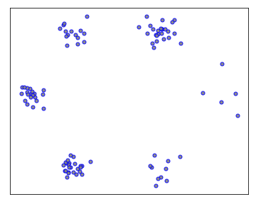
Let’s first look at these questions in the context of several classical unsupervised learning methods. The goal is to provide intuition on what influence functions should tell us in the unsupervised setting. Consider the following two-dimensional training data $X$ composed of six clusters.
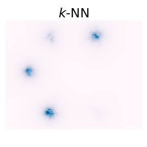
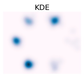
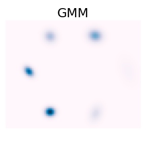
We consider three classical methods: the $k$-nearest-neighbour ($k$-NN) density estimator, the kernel density estimator (KDE), and Gaussian mixture models (GMM). We fit these models on $X$ and the probability densities of these models are shown below.
Self influences
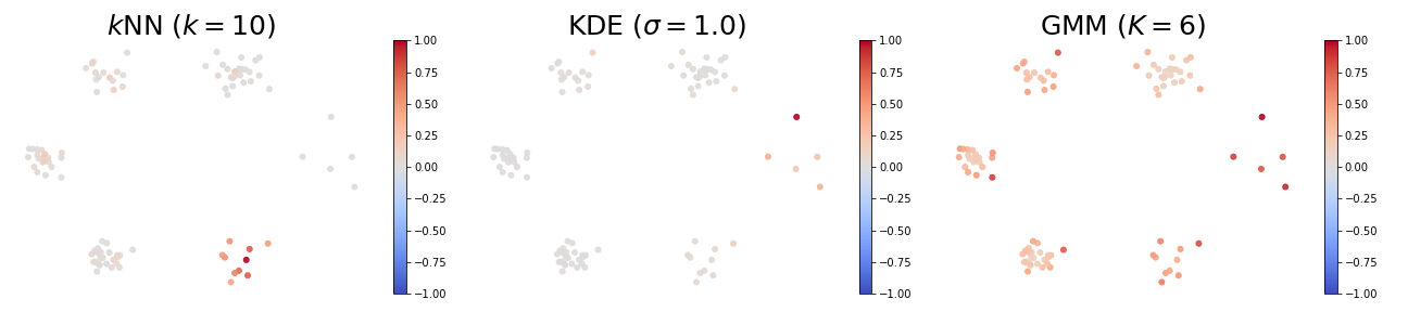
The figure below provides some insights of high and low self influence samples. The color of a point represents its self influence (red means high and blue means low).
- When using the $k$-NN density estimator, high self influence samples come from a cluster with exactly $k$ points.
- When using the KDE density estimator, high self influence samples come from sparse regions, and low self influence samples come from dense regions.
- When using the GMM density estimator, high self influence samples are far away to cluster centers, and low self influence samples are near cluster centers.
Proponents and Opponents
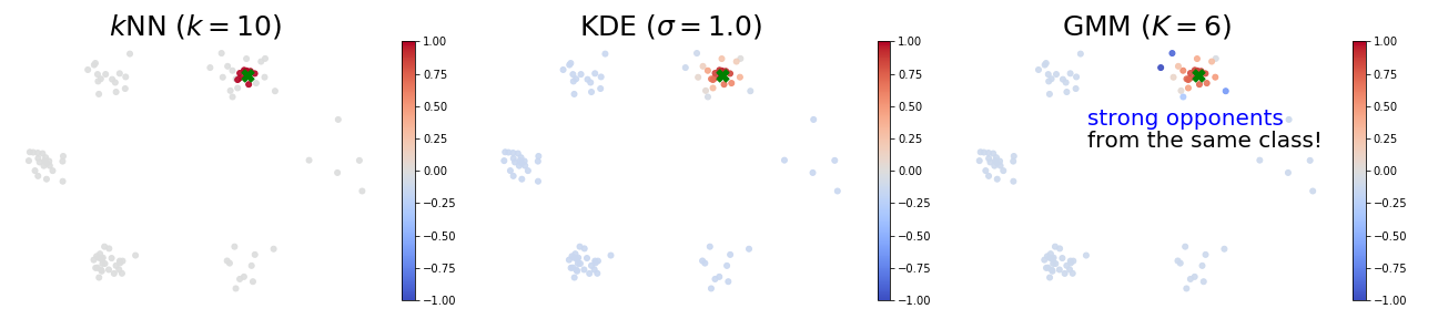
The figures below visualize an example of proponents and opponents. The test sample $z$ is marked as the green ✖︎ symbol, and the color of a point represents its influence over the test sample (red means proponents and blue means opponents). In all these models, strong proponents are the nearest neighbours of the test sample.
- When using the $k$-NN or the KDE density estimator, strong proponents of $z$ are exactly its $k$ nearest neighbours.
- KDE seems to be the soft version of $k$-NN: influences over $z$ gradually decrease as distances to $z$ increase.
- When using the GMM density estimator, it is surprising to observe that some strong opponents (blue points) of $z$ are from the same cluster! This phenomenon indicates that removing a sample from the same class can possibly increase the likelihood at $z$. To see why this happens, we note the GMM is parametric and has limited capacity. Therefore, training samples that are far away to the cluster centers can largely affect the mean and covariance matrices of the learned Gaussians.
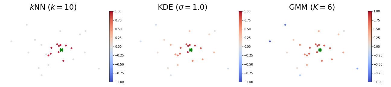
Scatter plots of influences of all training samples:
And the zoom in view that only shows the cluster which $z$ belongs to:
Note: please refer to Section 3 of our paper for the closed-form influence functions.
Variational Auto-Encoders (VAE)
Variational auto-encoders are a class of generative models composed of two networks: the encoder, which maps samples to latent vectors, and the decoder, which maps latent vectors to samples. These models are trained to maximize the evidence lower bound (ELBO), a lower bound of log-likelihood.
There are two challenges when we investigate influence functions in VAE.
- The influence function involves computing the loss at a test sample. However, the ELBO objective in VAE has an expectation term over the encoder, so it cannot be precisely computed.
- Solution: we compute the empirical average of the influence function. We provide a probabilistic error bound on this estimate: if the empirical average is over $\mathcal{\Theta}\left(\frac{1}{\epsilon^2\delta}\right)$ samples, then with probability at least $1-\delta$, the error between the empirical and true influence functions is no more than $\epsilon$.
- The influence function is hard to compute, as it requires inverting a large Hessian matrix. The number of rows in this matrix equals to the number of parameters in the VAE model, which can be as large as a million. Consequently, inverting this matrix (or even computing Hessian vector products) can be computationally infeasible.
- Solution: we propose a computationally efficient algorithm called VAE-TracIn. It is based on the fast TracIn algorithm, an approximation to influence functions. TracIn is efficient because (1) it only involves computing the first-order derivative of the loss, and (2) it can be accelerated with only a few checkpoints.
A sanity check
Does VAE-TracIn find the most influential training samples? In a good instance-based interpretation, training samples should have large influences over themselves. Therefore, we design the following sanity check (which is analogous to the identical subclass test by Hanawa et al. in this reference):
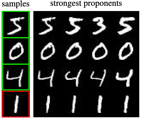
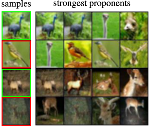
The short answer is: yes. We visualize some training samples and their strongest proponents in the figures below. A sample is marked in a green box if it is exactly its strongest proponent, and in a red box otherwise. Quantitatively, almost all ($>99\%$) training samples are the strongest proponents of themselves, with only very few exceptions. And as shown, even if a samples is not its strongest proponent, it still ranks very high in the order of influence scores.
Self influences for VAEs
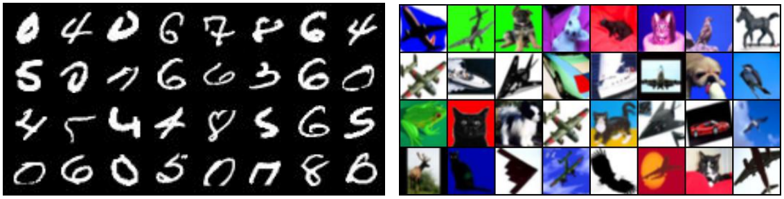
We visualize high self influence samples below. We find these samples are either hard to recognize or visually high-contrast.
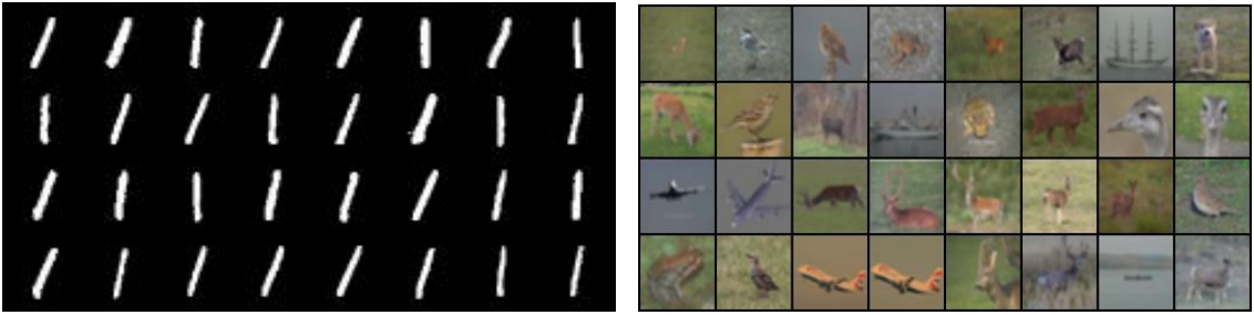
We then visualize low self influence samples below. We find these samples share similar shapes or background.
These findings are consistent with the memorization analysis in the supervised setting by Feldman and Zhang in this reference. Intuitively, high self influence samples are very different from most samples, so they must be memorized by the model. Low self influence samples, on the other hand, are very similar to each other, so the model does not need to memorize all of them. Quantitatively, we also find self influences correlate to the loss of training samples: generally, the larger loss, the larger self influence.
The intuition on self influences leads to an application in unsupervised data cleaning. Because high self influence samples are visually complicated and different, they are likely to be outside the data manifold. Therefore, we can use self influences to detect unlikely (noisy, contaminated, or even incorrectly collected) samples. For example, they could be unrecognizable handwritten digits or objects in MNIST or CIFAR. Similar approaches in supervised learning use self influences to detect mislabeled data or memorized samples.
Proponents and Opponents in VAEs
We visualize strong proponents and opponents of several test samples below.
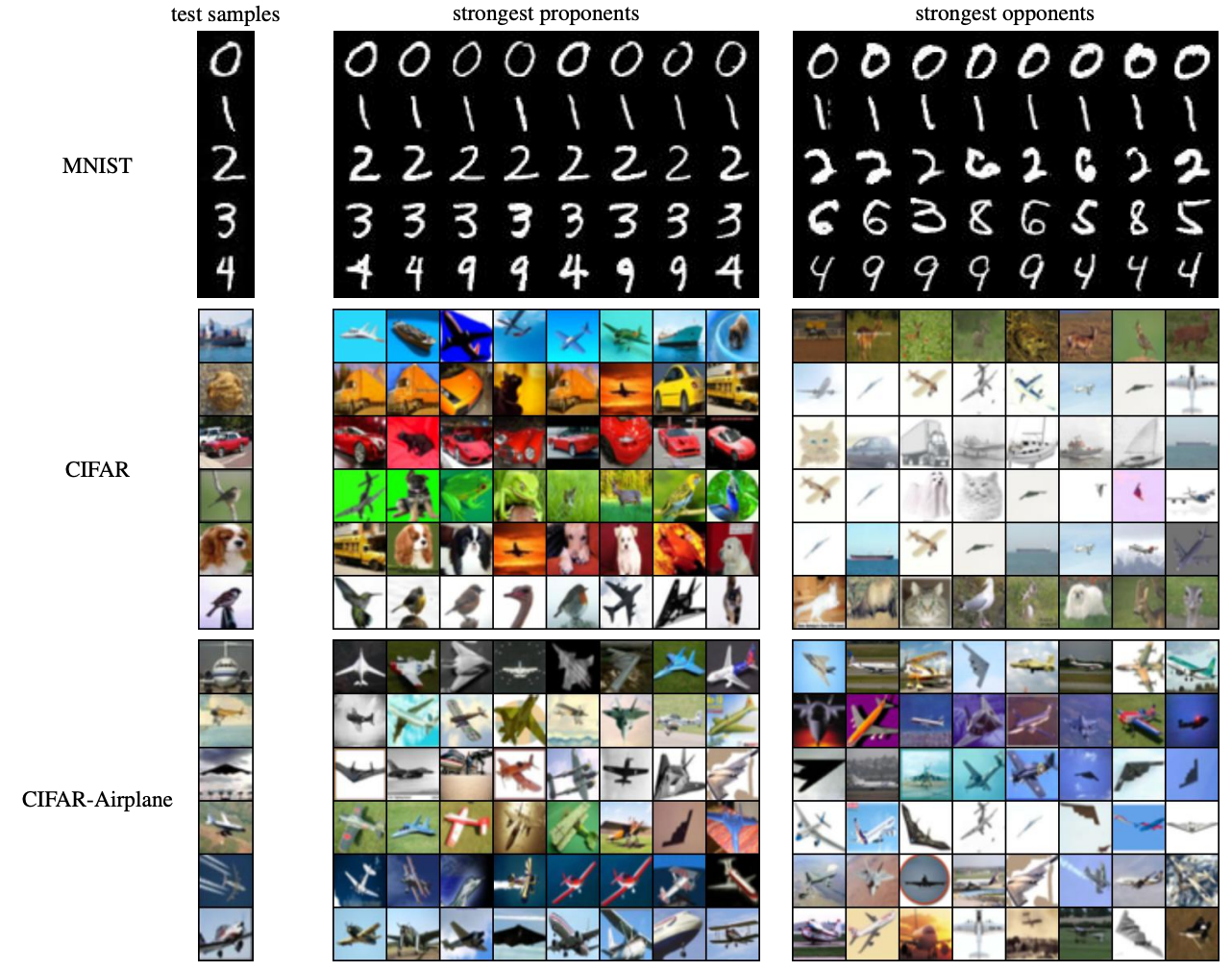
In MNIST, many strong proponents and opponents of test samples are similar samples from the same class. Especially, strong proponents look very similar to test samples, and strong opponents are visually slightly different. For example, the opponents of the test “two” have very different thickness and styles. Quantitatively, $\sim 80\%$ of the strongest proponents and $\sim 40\%$ of the strongest opponents have the same label as test samples. In addition, both of them have small latent space distance to the test samples. One can find this is very similar to GMM.
In CIFAR, we find strong proponents seem to match the color of the images – including the background and the object – and they tend to have the same but brighter colors. Strong opponents, on the other hand, tend to have very different colors as the test samples. Quantitatively, strong proponents have large norms in the latent space, indicating they are very likely to be outliers, high-contrast samples, or very bright samples. This observation is also validated in the visualizations. One can further connect this observation to influence functions in supervised learning. Hanawa et al. find extremely large norm samples are selected as relevant instances by influence functions in this reference, and Barshan et al. find large norm samples can impact a large region in the data space when using the logistic regression in this reference.
Open Questions
There are many open questions based on our paper. Here is a list of some important future directions.
- How to design efficient instance-based interpretation methods for modern, large unsupervised learning models trained on millions of samples?
- How can we use the instance-based interpretations to detect biases and fairness in models and data?
- What are the other applications of instance-based interpretation methods?