Connecting Interpretability and Robustness in Decision Trees through Separation
TL;DR We construct a tree-based model that is
Imagine a world where computers are fully integrated into our everyday lives. Making decisions independently, without human intervention. No need to worry about overly exhausted doctors making life-changing decisions or driving your car after a long day at the office. Sounds great, right? Well, what if those computers weren’t reliable? What if a computer decided you need to go through surgery without telling you why? What if a car confused a child with a green light? It doesn’t sound so great after all.
Before we fully embrace machine learning, it needs to be reliable. The cornerstones for reliable machine learning are (i) interpretability, where the model’s decisions are transparent, and (ii) robustness, where small changes to the input do not change the model’s prediction. Unfortunately, these properties are generally studied in isolation or only empirically. Here, we explore interpretability and robustness simultaneously, and examine it both theoretically and empirically.
We start this post by explaining what we mean by interpretability and robustness. Next, to derive guarantees, we need some assumptions on the data. We start with the known $r$-separated data. We show that although there exists a tree that is accurate and robust, such tree can be exponentially large, which makes it not interpretable. To improve the guarantees, we make a stronger assumption on the data and focus on linearly separable data. We design an algorithm called BBM-RS and prove that it is accurate, robust, and interpretable on linearly separable data. Lastly, real datasets may not be linearly separable, so to understand how BBM-RS performs in practice, we conduct an empirical study on $13$ datasets. We find out that BBM-RS brings better robustness and interpretability while performing competitively on test accuracy.
What do we mean by interpretability and robustness?
Interpretability
A model is interpretable if the model is simple and self-explanatory. There are several forms of self-explanatory models, e.g., decision sets, logistic regression, and decision rules. One of the most fundamental interpretable models, which we focus on here, are small decision trees. We use the size of a tree to determine whether it is interpretable or not.
Robustness
We also want our model to be robust to adversarial perturbations.
This means that if example $x$ is changed, by a bit, to $x’$, the model’s
answer remains the same.
By “a bit”, we mean that $x’=x+\delta$ where $\|\delta\|_\infty\leq r$ is
small. A model $h:\mathbf{X} \rightarrow \{-1, +1\}$ is
Guarantees under different data assumptions
Without any assumptions on the data, we cannot guarantee accuracy, interpretability, and robustness to hold simultaneously. For example, if the true labels of the examples are different for close examples, a model cannot be astute (accurate and robust). In this section, we explore which data properties are sufficient for astuteness and interpretability.
$r$-Separation
A prior work suggested
focusing on datasets that satisfy $r$-separation.
A binary labeled data distribution is
Linear separation
Next, we investigate a stronger assumption — linear separation with a $\gamma$-margin. Intuitively, it means that a hyperplane separates the two labels in the data, and the margin (distance of the closest point to the hyperplane) is at least $\gamma$ (larger $\gamma$ means larger margin for the classifier). More formally, there exists a vector $w$ with $\|w\|_1=1$ such that for each training example and its label $(x, y)$, we have $ywx\geq \gamma$. Linear separation is a popular assumption in the research of machine learning models, e.g., for support vector machines, neural networks, and decision trees.
Using a generalization of previous work, we know that under the linear separation assumption, there has to be a feature that gives nontrivial information. To formalize it, we use the notion of decision stumps and weak learners. A decision stump is a (simple) hypothesis of the form $sign(x_i-\theta)$ defined by a feature $i$ and a threshold $\theta$. A hypothesis class is a $\gamma$-weak learner if one can learn it with accuracy $\gamma$ (slightly) better than random, i.e., if there is always a hypothesis in the class with accuracy of at least $1/2+\gamma$.
Now, we look at the hypothesis class of all possible decision stumps, and we want to show that this class is a weak learner. For each dataset $S=((x^1,y^1),\ldots,(x^m,y^m))$, we denote the best decision stump for this dataset by $h_S(x)=sign(x_i-\theta)$, where $i$ is a feature and $\theta$ is a threshold that minimize the error $\sum_{j=1}^m sign(x^j_i < \theta) y^j.$ We can show that $h_S$ has accuracy better than $0.5$, i.e., better than a random guess:
This result proves that there exists a classifier $h_S$ in the hypothesis class of
all possible decision stumps that produces a non-trivial
solution under the linear separability assumption.
Using this theorem along with the result from
Kearns and Mansour,
we can show that
CART-type
algorithms can deliver a small tree with high accuracy.
As a side benefit, this is the
Are we done? Is this model also robust?
New algorithm: BBM-RS
Designing robust decision trees is inherently a difficult task. One reason is that, generally, the models defined by the right and left subtrees can be completely different. The feature $i$ in the root determines if the model uses the right or left subtree. Thus, a small change in the $i$-th feature completely changes the model. To overcome this difficulty, we focus on a specific class of decision trees.
Risk score
We design our algorithm to learn a specific kind of decision tree — risk score. A risk score is composed of several conditions (e.g., $age \geq 75$), and each is matched with an integer weight. A score $s(x)$ of example $x$ is the weighted sum of all the satisfied conditions. The label is then $sign(s(x))$.
| features | weights | |
|---|---|---|
| Bias term | -5 | + ... |
| Age $\geq 75$ | 2 | + ... |
| Called before | 4 | + ... |
| Previous call was successful | 2 | + ... |
| total scores= | ||
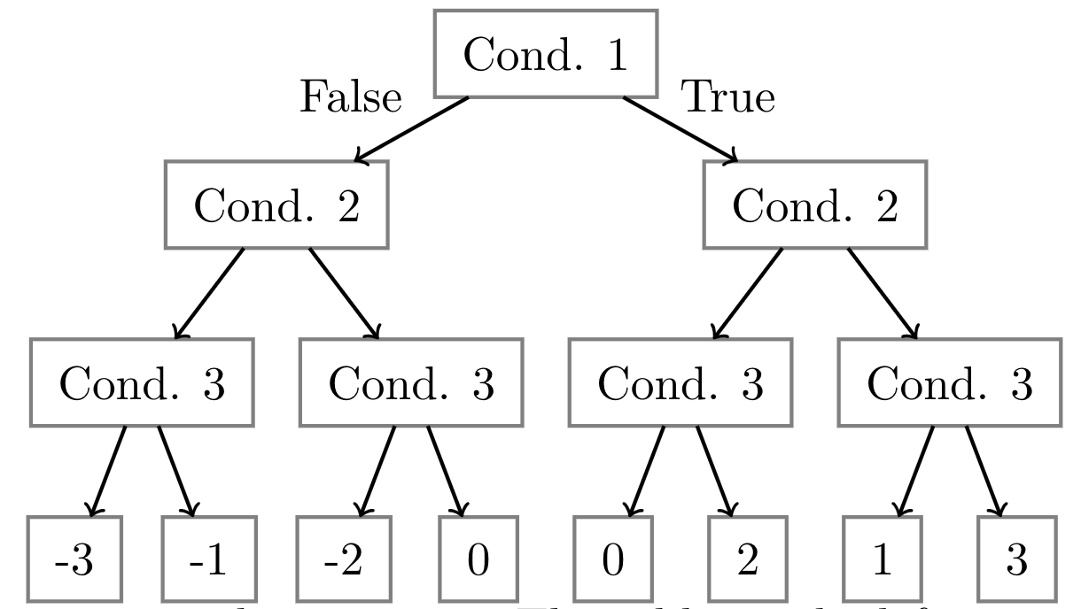
A risk score can be viewed as a decision tree with the same feature-threshold pair at each level (see example below). A risk score has simpler structure than a standard decision tree, and it generally has fewer number of unique nodes. Hence, they are considered more interpretable than decision trees. The following table shows an example of a risk score.
| features | weights | |
|---|---|---|
| Bias term | -3 | + ... |
| Fever | 3 | + ... |
| Sneeze | 1 | + ... |
| Cough | 2 | + ... |
| total scores= |
BBM-RS
We design a new algorithm for learning risk scores by utilizing the known boosting method boost-by-majority (BBM). The different conditions are added to the risk score one by one, using the weak learner. BBM has the benefit of ensuring the weights in the risk score are small integers. This will lead to an interpretable model with size only $O(\gamma^{-2}\log1/\epsilon)$ where the model has accuracy $1-\epsilon$.
Now we want to make sure that the risk model is also robust. The idea is to add noise. We take each point in the sample and just make sure that it’s a little bit closer to the decision boundary, see the figure below.
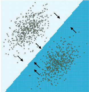
The idea is that if the model is correct for the noisy point, then it should be correct for the point without the noise. To formally prove it, we show that choosing the risk-score conditions in a specific way ensures that they are monotone models. In such models, adding noise in the way we described is sufficient for robustness.
Before we examine this algorithm on real datasets, let’s check its running time. We focus on the case the margin and desired accuracy are constants. In this case, the number of steps BBM-RS will take is also constant. In each step, we run the weak learner and find the best $(i,\theta)$. So the overall time is linear (up to logarithmic factors) in the input size and the time to run the weak learner.
To summarize, we designed a new efficient algorithm, BBM-RS, that is robust, interpretable, and has high accuracy. The following theorem shows this. Please refer to our paper for the pseudocode of BBM-RS and more details for the theorem.
Performance on real data
For BBM-RS, our theorem is restricted to linearly separable data. However, real datasets may not perfectly linearly separable. A straightforward question: is linear separability a reasonable assumption in practice?
To answer this question, we consider $13$ real datasets (here we present the results for four datasets; for more datasets, please refer to our paper). We measure how linearly separable each of these datasets is. We define the linear separateness as one minus the minimal fraction of points that needed to be removed for the data to be linearly separable. Since finding the optimal linear separateness on arbitrary data is NP-hard, we approximate linear separateness with the training accuracy of the best linear classifier we can find (since removing the incorrect examples for a linear classifier would make the dataset linearly separable). We train linear SVMs with different regularization parameters and record the best training accuracy. After removing the misclassified points by an SVM, we are left with accuracy fraction of linearly separable examples. The higher this accuracy is, the more linearly separable the data is. The following table shows the results and it reveals that most datasets are very or moderately close to being linearly separated. This indicates that the linear assumption in our theorem may not be too restrictive in practice.
| linear separateness | |
|---|---|
| adult | 0.84 |
| breastcancer | 0.97 |
| diabetes | 0.77 |
| heart | 0.89 |
Even though these datasets are not perfectly linearly separable, BBM-RS can still be applied (but the theorem may not hold). We are interested to see how BBM-RS performed against others on these non-linearly separable datasets. We compare BBM-RS to three baselines, LCPA, decision tree (DT), and robust decision tree (RobDT). We measure a model’s robustness by evaluating its Empirical robustness (ER), which is the average $\ell_\infty$ distance to the closest adversarial example on correctly predicted test examples. The larger ER is, the more robust the classifier is. We measure a model’s interpretability by evaluating its interpretation complexity (IC). We measure IC with the number of unique feature-threshold pairs in the model (this corresponds to the number of conditions in the risk score). The smaller IC is, the more interpretable the classifier is. The following tables show the experimental results.
| test accuracy (higher=better) | ||||
|---|---|---|---|---|
| DT | RobDT | LCPA | BBM-RS | |
| adult | 0.83 | 0.83 | 0.82 | 0.81 |
| breastcancer | 0.94 | 0.94 | 0.96 | 0.96 |
| diabetes | 0.74 | 0.73 | 0.76 | 0.65 |
| heart | 0.76 | 0.79 | 0.82 | 0.82 |
| ER (higher=better) | ||||
|---|---|---|---|---|
| DT | RobDT | LCPA | BBM-RS | |
| adult | 0.50 | 0.50 | 0.12 | 0.50 |
| breastcancer | 0.23 | 0.29 | 0.28 | 0.27 |
| diabetes | 0.08 | 0.08 | 0.09 | 0.15 |
| heart | 0.23 | 0.31 | 0.14 | 0.32 |
| IC feature threshold pairs (lower=better) | ||||
|---|---|---|---|---|
| DT | RobDT | LCPA | BBM-RS | |
| adult | 414.20 | 287.90 | 14.90 | 6.00 |
| breastcancer | 15.20 | 7.40 | 6.00 | 11.00 |
| diabetes | 31.20 | 27.90 | 6.00 | 2.10 |
| heart | 20.30 | 13.60 | 11.90 | 9.50 |
From the tables, we see that BBM-RS has a test accuracy comparable to other methods. In terms of robustness, it performs slightly better than others (performing the best on three datasets among a total of four). In terms of interpretability, BBM-RS performs the best in three out of four datasets. All in all, we see that BBM-RS can bring better robustness and interpretability while performing competitively on test accuracy. This shows that BBM-RS not only performs well theoretically, it also performs well empirically.
Conclusion
We investigated three important properties of a classifier: accuracy, robustness, and interpretability. We designed and analyzed a tree-based algorithm that provably achieves all these properties, under linear separation with a margin assumption. Our research is a step towards building trustworthy models that provably achieve many desired properties.
Our research raises many open problems. What is the optimal dependence between accuracy, interpretation complexity, empirical robustness, and sample complexity? Can we have guarantees using different notions of interpretability? We showed how to construct an interpretable, robust, and accurate model. But, for reliable machine learning models, many more properties are required, such as privacy and fairness. Can we build a model with guarantees on all these properties simultaneously?
More Details
See our paper on arxiv or our repository.