The Expressive Power of Normalizing Flow Models
Background: Generative Models and Normalizing Flows
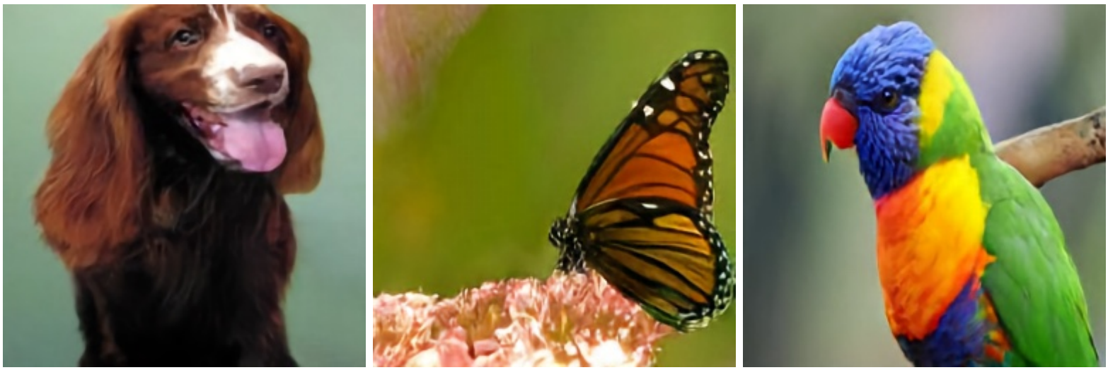
Generative models are one kind of unsupervised learning model in machine learning. Given a set of training data – such as pictures of dogs, audio clips of human speakers, and articles from certain websites – a generative model aims to generate samples that look/sound like they are samples from the dataset, but are not exactly any one of them. We usually train a generative model by maximizing the probability, or likelihood, of the samples under the model.
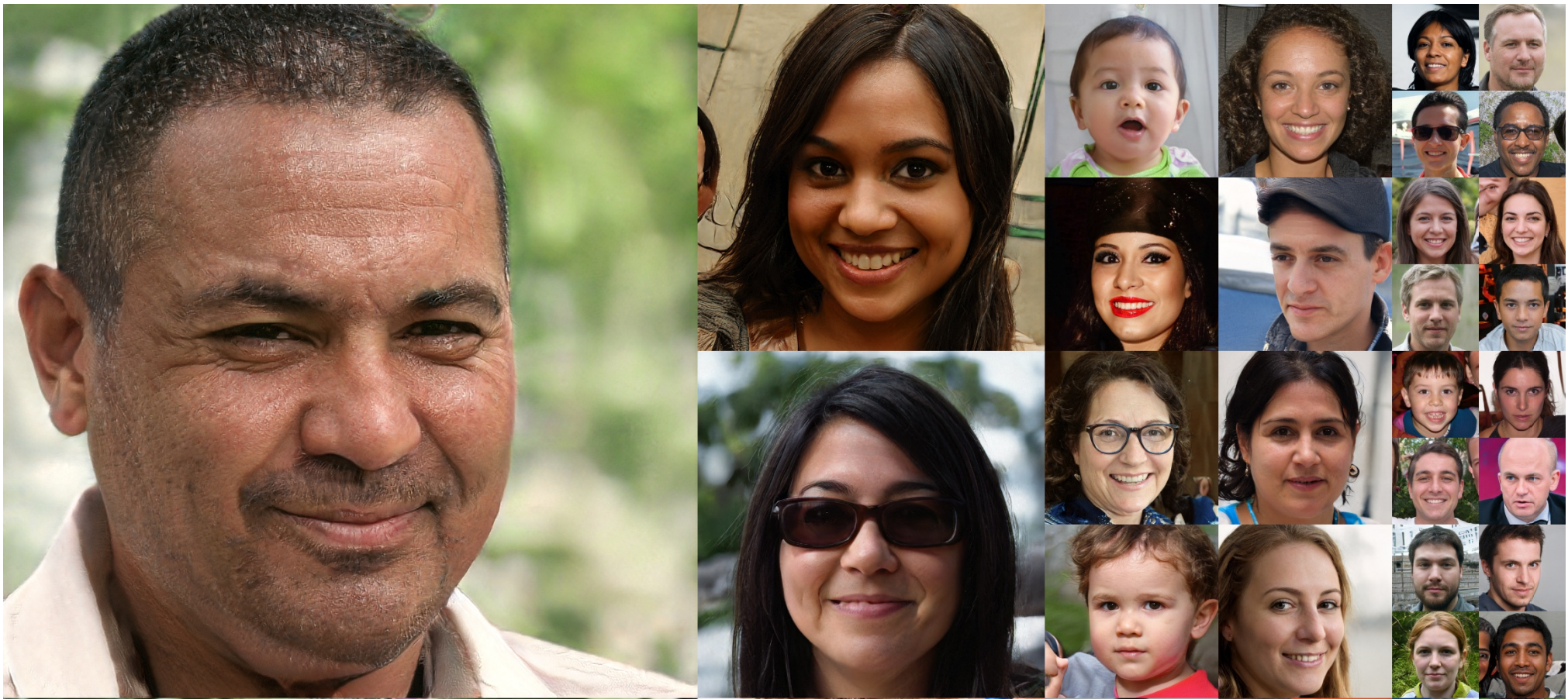
To understand complicated training data, generative models usually use very large neural networks (so they are also called deep generative models). Popular deep generative models include generative adversarial networks (GANs) and variational autoencoders (VAEs), which have achieved the state-of-the-art performances on most generative tasks. Below are examples showing that styleGAN (left) and VQ-VAE (right) can generate amazing high resolution images!
One might ask: as we already have powerful generative models, is everything done? No! There are many aspects in which we want to improve these models. Below are two points related to this blog.
First, we want to compute exact likelihood if possible. Both GANs and VAEs generate samples by applying a neural network transformation on a latent random variable $z$, which is usually a Gaussian. In this case, the sample likelihood cannot be exactly computed because complicated neural networks may map different $z$’s to the same output.
This is the reason why normalizing flows (NFs) were proposed. An NF learns an invertible function $f$ (which is also a neural network) to convert a source distribution, such as a Gaussian, to the distribution of the training data. Since $f$ is invertible, we can precisely compute the likelihood through the change-of-variable formula! This post includes the detailed math of the computation. Different from the decoder in VAEs and the generator in GANs (which usually transform a lower dimensional latent variable to the data distribution), the NF $f$ keeps the data dimension and $f^{-1}$ can map a sample back to the source distribution.
Second, we want a theoretical guarantee that these deep generative models are potentially able to learn an arbitrarily complicated data distribution. Without such theory, an empirically successful generative model might fail in another scenario, and we don’t want this risk to always exist! Despite its importance, this problem is super challenging due to the complicated structure of neural networks. For example, this paper analyzes GANs in transforming between very simple distributions.
This blog addresses the above two points by making a theoretical analysis to NFs. We provide a theoretical guarantee for NFs on $\mathbb{R}$ and some negative (impossibility) results for NFs on $\mathbb{R}^d$ where the dimension $d>1$.
Structure of Normalizing Flows
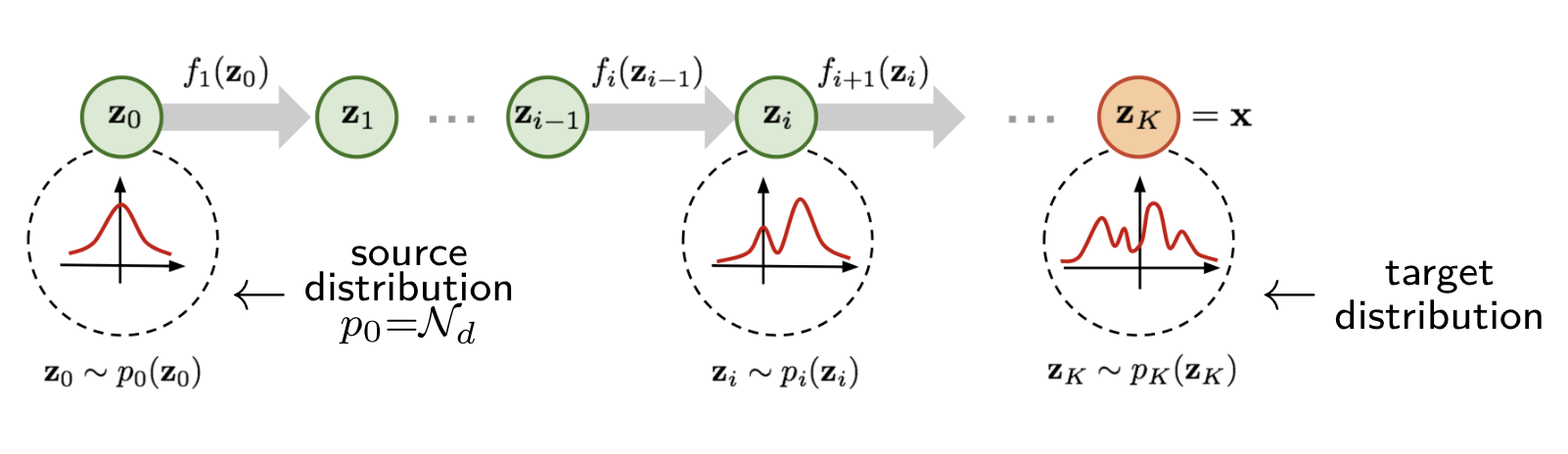
In general, to model complex training data like images, the normalizing flow $f$ needs to be a very complicated function. In practice, $f$ is usually constructed via a sequence of simple, invertible transformations, which we call base flow layers. The figure below illustrates the middle stages within the transformation from a simple source distribution to a complicated target distribution (figure from this link).
Examples of base flow layers include
-
planar layers: $f_{\text{pf}}(z)=z+uh(w^{\top}z+b)$, where $u,w,z\in\mathbb{R}^d,b\in\mathbb{R}$;
-
radial layers: $f_{\text{rf}}(z)=z+\frac{\beta}{\alpha+\|z-z_0\|}(z-z_0)$, where $z,z_0\in\mathbb{R}^d,\alpha,\beta\in\mathbb{R}$;
-
Sylvester layers: $f_{\text{syl}}(z)=z+Ah(B^{\top}z+b)$, where $A,B\in\mathbb{R}^{d\times m}, z\in\mathbb{R}^d, b\in\mathbb{R}^m$;
-
and Householder layers: $f_{\text{hh}}(z)=z-2vv^{\top}z$, where $v,z\in\mathbb{R}^d, v^{\top}v=1$.
The number of layers is usually very large in practice. For instance, in the MNIST dataset experiments, this paper uses 80 planar layers, and this paper uses 16 Sylvester layers.
Defining the Expressivity of Normalizing Flows
The invertibility of NFs may hugely restrict their expressive power, but to what extent? Our recent paper analyzes this through the following two questions:
-
Q1 (Exact transformation): Under what conditions is it possible to exactly transform the source distribution $q$ (e.g., a standard Gaussian) into the target distribution $p$ with a finite number of base flow layers?
-
Q2 (Approximation): Since sometimes exact transformation may be hard, when is it possible to approximate the target distribution $p$ in total variation distance? Do we need an incredibly large number of layers?
Our findings:
-
If $p$ and $q$ are defined on $\mathbb{R}$, then universal approximation can be achieved. That is, we can always transform $q$ to be arbitrarily close to any $p$.
-
If $p$ and $q$ are defined on $\mathbb{R}^d$ where $d>1$, both exact transformation and approximation may be hard. Having a large number of layers is a necessary (but not a sufficient) condition.
Challenges
Our problem is very related to the universal approximation property: the ability of a function class to be arbitrarily close to any target function. Although we have this property for shallow neural networks, fully connected networks, and residual networks, these results do not apply to NFs. Why? Because of the invertibility.
-
First, a function class has the universal approximation property does not imply that its invertible subset can approximate between any pair of distributions. For instance, take the set of piecewise constant functions. Its invertible subset is the empty set!
-
On the other hand, a function class has limited capacity does not imply that its invertible subset cannot transform between any pair of distributions. For instance, take the set of triangular maps, which can perform powerful Knothe–Rosenblatt rearrangements (See page 17 of this book).
The way to get around this challenge: instead of looking at the capacity of a function class in the function space, we directly analyze input–output distribution pairs.
Universal Approximation When $d=1$
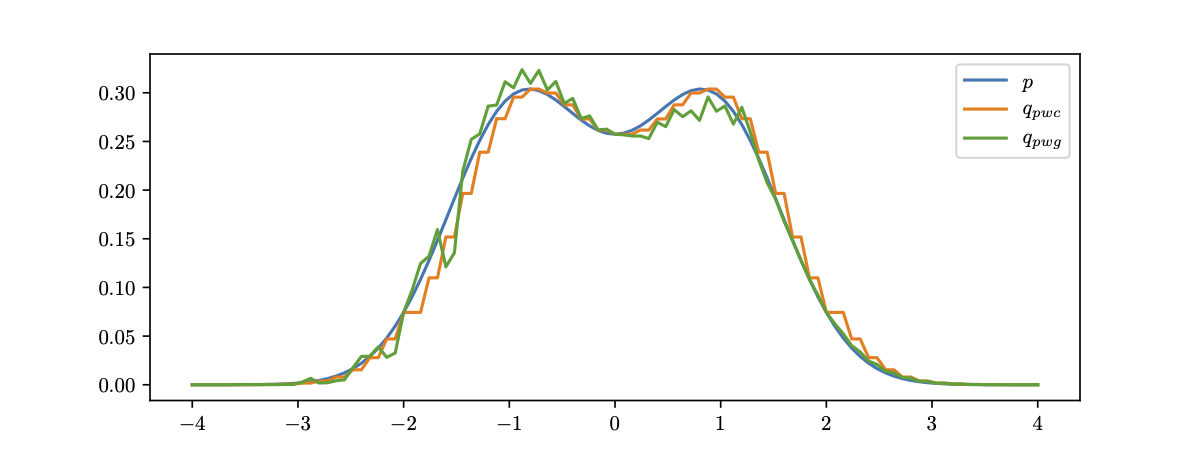
As warm-up let us look at the one-dimensional case. We show planar layers can approximate between arbitrary pairs of distributions under mild assumptions. We analyze a specific kind of planar layer with the ReLU activation: \[f_{\text{pf}}(z)=z+u\ \mathrm{ReLU}(wz+b)\] where $u,w,b,z\in\mathbb{R}$, and $\text{ReLU}(x)=\max(x,0)$. The effect of this transformation on a density is first splitting its graph into two pieces, and then scaling one piece while keeping the other one unchanged. For example, in the figure below the first planar layer splits the blue line into the solid part and the dashed part, and scales the dashed part to the orange line. Similarly, the second planar layer splits the orange line into the solid part and the dashed part, and scales the dashed part to the green line.
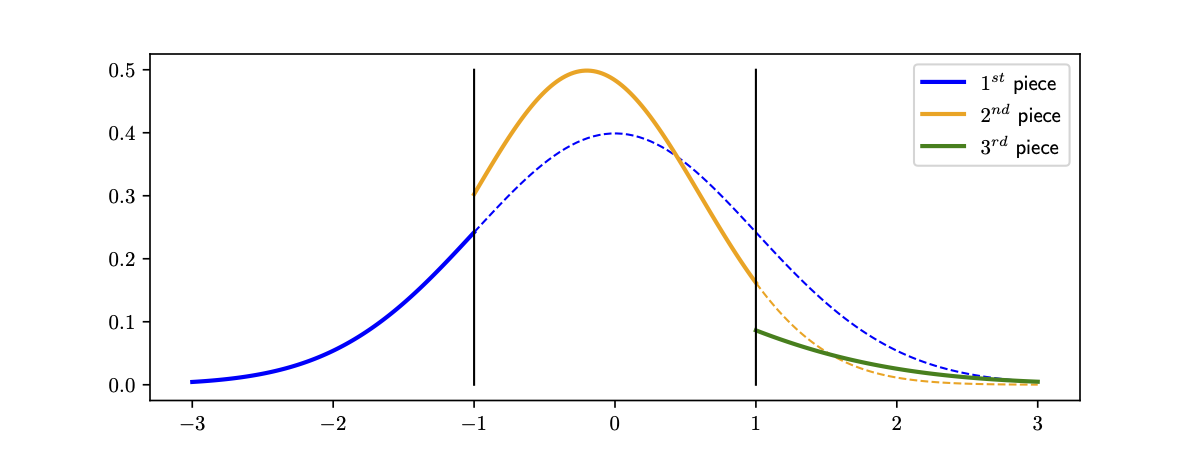
In particular, if the blue line is Gaussian, then the orange line and the green line are also pieces of some Gaussian distributions. We call this a piecewise Gaussian distribution. Additionally, it has the consistency property: the integration of the transformed distribution should always be 1.
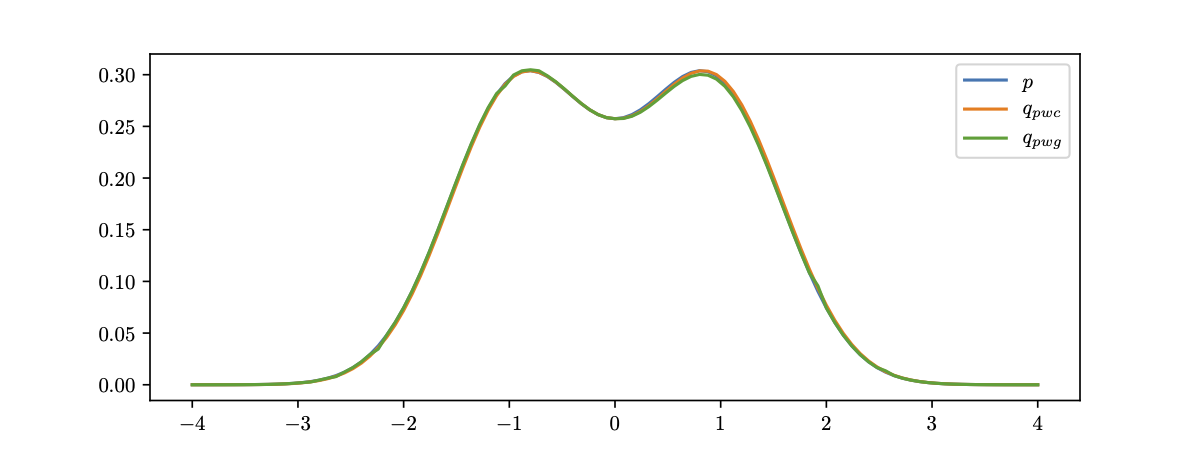
How does it relate to approximation? Here we use a fundamental result in real analysis: Lebesgue-integrable functions can be approximated by piecewise constant functions. Given a piecewise constant distribution $q_{\text{pwc}}$ that is close to the target distribution $p$, we can iteratively construct a piecewise Gaussian distribution $q_{\text{pwg}}$ with the same group of pieces. We can additionally require $q_{\text{pwg}}$ to be very close to $q_{\text{pwc}}$ by carefully selecting the parameters $u,w,b$. Finally, as the pieces become smaller, $q_{\text{pwc}}\rightarrow p$ and $q_{\text{pwg}}\rightarrow q_{\text{pwc}}$, which implies $q_{\text{pwg}}\rightarrow p$.
In the following example, we demonstrate such approximation with 50(top) and 300(bottom) ReLU planar layers, respectively.
Exact Transformation When $d>1$
Next, we look at the more general case in higher-dimensional space, which is usually quite different from the one-dimensional case. We show exact transformation between distributions can be quite hard. Specifically, we analyze Sylvester layers, a matrix-form generalization of planar layers (note that on $\mathbb{R}$, planar layers and Sylvester layers are equivalent): \[f_{\text{syl}}(z)=z+Ah(B^{\top}z+b)\] where $A,B\in\mathbb{R}^{d\times m},z\in\mathbb{R}^d,b\in\mathbb{R}^m$ for some integer $m$. In particular, we call $m$ the number of neurons of $f_{\text{syl}}$ because its form is identical to a residual block with $m$ neurons in the hidden layer.
Now suppose we stack a number of Sylvester layers with $M$ neurons in total, and these layers sequentially transform an input distribution $q$ to output distribution $p$. For convenience, let $f$ be the function composed of all these Sylvester layers. We show that the distribution pairs $(q,p)$ must obey some necessary (but not sufficient) condition, which we call the topology matching condition.
- $h$ is a smooth function
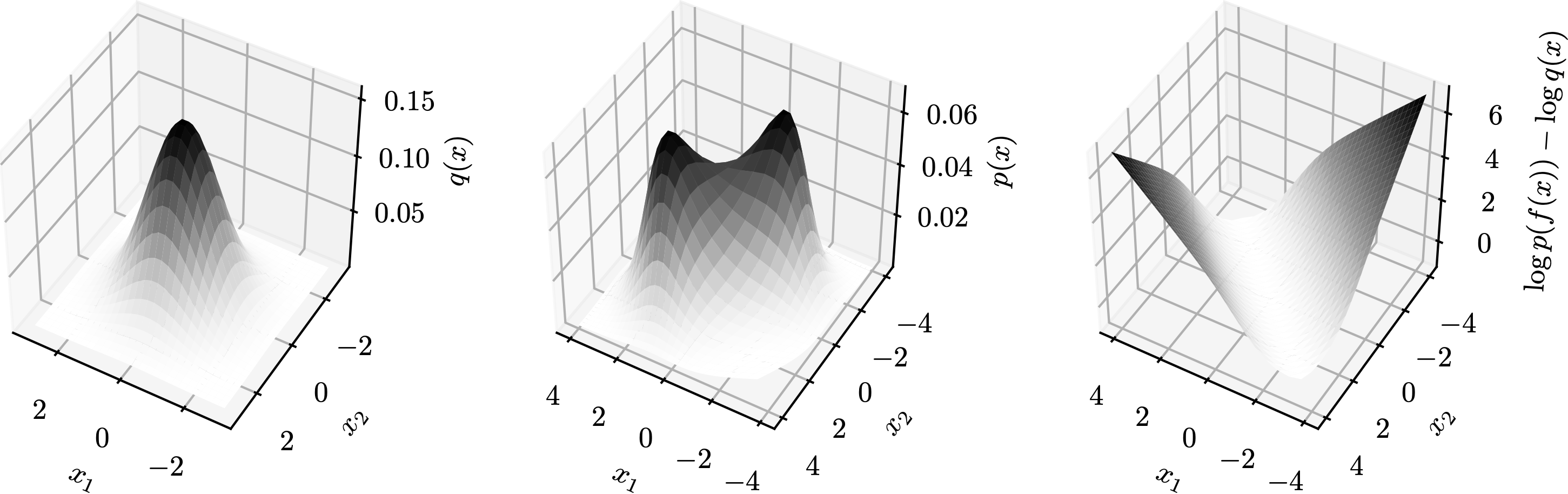
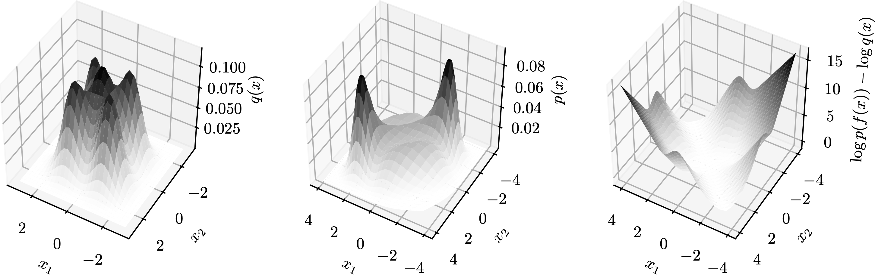
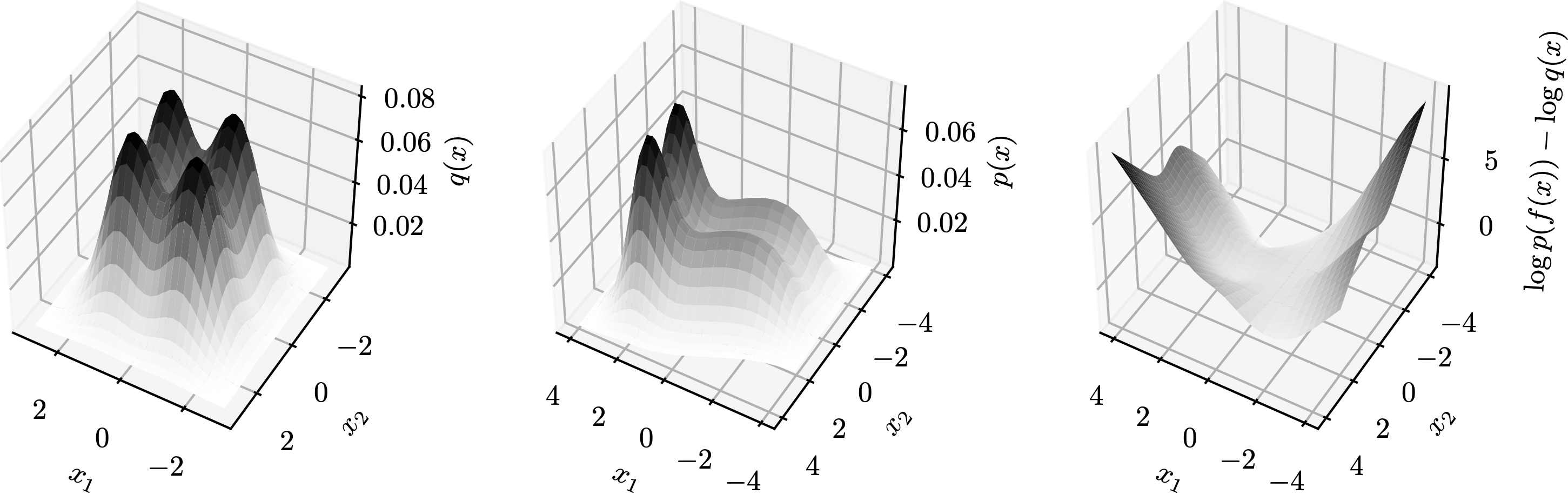
Let $L(z)=\log p(f(z))-\log q(z)$ be the log-det Jacobian term. Then, the topology matching condition says the dimension of the set of the gradient of $L$ is no more than the number of neurons. Formally, \[\dim\{\nabla_z L(z):z\in\mathbb{R}^d\}\leq M\] In other words, if $M$ is less than the above dimensionality then exact transformation is impossible no matter what smooth non-linearities $h$ are selected. Since it is not easy to plot $\{\nabla_z L(z):z\in\mathbb{R}^d\}$, we demonstrate $L(z)$ in a few examples below. Each row is a group, containing plots of $q$, $p$, and $L$ from left to right. In these examples, $M=1$ so $\nabla_z L(z)$ is a multiple a constant vector.
→ 
→ 
→ 
→ 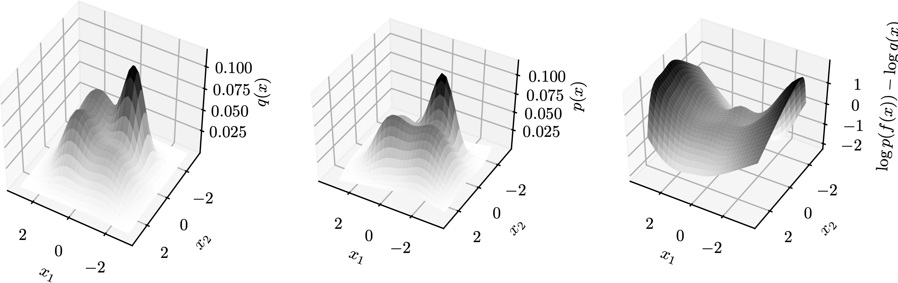
Based on the topology matching condition, it can be shown that if the number of neurons $M$ is less than the dimension $d$, it may even be hard to transform between simple Gaussian distributions.
- When $h=\text{ReLU}$
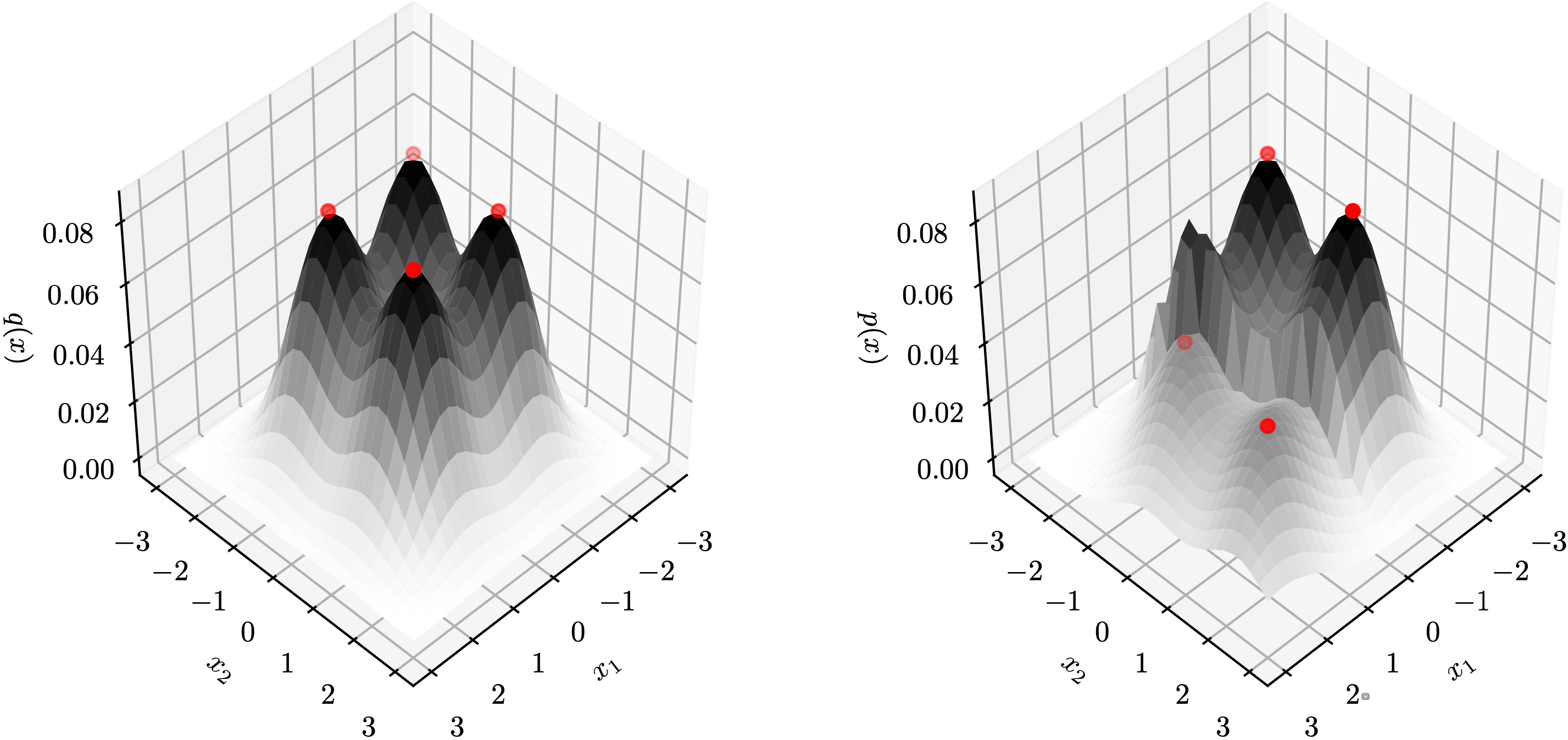
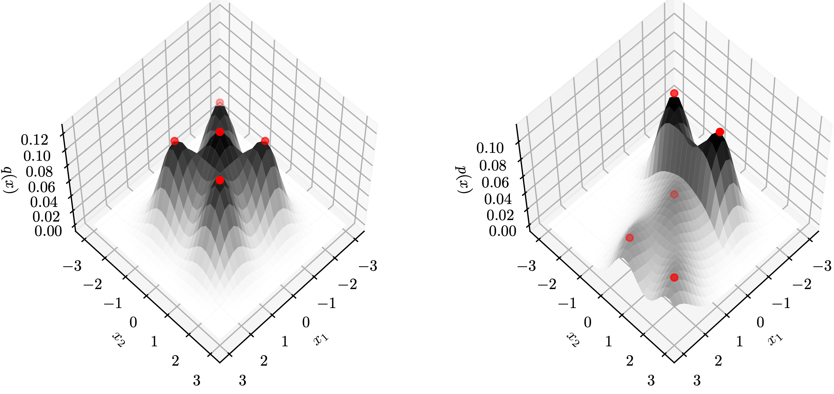
We then restrict to ReLU Sylvester layers. In this case, $f$ in fact performs a piecewise linear transformation in $\mathbb{R}^d$. As a result, for almost every $z\in\mathbb{R}^d$ (except for boundary points), $f$ is linear around $z$. This leads to the following (pointwise) topology matching condition: there exists a constant matrix $C$ (which is the Jacobian matrix of $f(z)$) around $z$ such that \[C^{\top}\nabla_z\log p(f(z))=\nabla_z\log q(z)\]
We demonstrate this result with two examples below, where each row is a $(q,p)$ distribution pair. The red points ($z$) on the left are transformed to those ($f(z)$) on the right by $f$. Notice that these red points are peaks of $q$ and $p$, respectively. In these cases, both $\nabla_z\log p(f(z))$ and $\nabla_z\log q(z)$ are zero vectors, which is compatible with the topology matching condition.
→ 
→ 
As a corollary, we conclude that ReLU Sylvester layers generally do not transform between product distributions or mixture of Gaussian distributions except for very special cases.
Approximation Capacity When $d>1$
It is not surprising that exact transformation between distributions is difficult. What if we loosen our goal to approximation between distributions, where we can use transformations from a certain class $\mathcal{F}$? We show that unfortunately, this is still hard under certain conditions.
The way to look at this problem is to bound the minimum depth that is needed to approximate between $q$ and $p$. In other words, if we use less than this number of transformations, then it is impossible to approximate $p$ given $q$ as the source, no matter what transformations in $\mathcal{F}$ are selected. Formally, for $\epsilon>0$, we define the minimum depth as \[T_{\epsilon}(p,q,\mathcal{F})=\inf\{n: \exists \{f_i\}_{i=1}^n\in\mathcal{F}\text{ such that }\mathrm{TV}((f_1\circ\cdots\circ f_n)(q),p)\leq\epsilon\}\] where $\mathrm{TV}$ is the total variance distance.
We conclude that if $\mathcal{F}$ is the set of $(i)$ planar layers $f_{\text{pf}}$ with bounded parameters and popular non-linearities including $\tanh$, sigmoid, and $\arctan$, or $(ii)$ all Householder layers $f_{\text{hh}}$, then $T_{\epsilon}(p,q,\mathcal{F})$ is not small. In detail, for any $\kappa>0$, there exists a pair of distributions $(q,p)$ on $\mathbb{R}^d$ and a constant $\epsilon$ (e.g., 0.5) such that \[T_{\epsilon}(p,q,\mathcal{F})=\tilde{\Omega}(d^{\kappa})\] Although this lower bound is polynomial in the dimension $d$, in many practical problems the dimension can be very large so the minimum depth is still an incredibly large number. This result tells us that planar layers and Householder layers are provably not very expressive under certain conditions.
Open Problems
This is the end of our paper, but is clearly just the beginning of the story. There are a large number of open problems on the expressive power of even simple normalizing flow transformations. Below are some potential directions.
- Just like neural networks, planar and Sylvester layers use non-linearities in their expressions. Is it possible that a certain combination of non-linearities (at different layers) can significantly improve capacity?
- Our paper does not provide a result for very deep Sylvester flows (e.g., $>d$ layers) with smooth non-linearities. Therefore, it is interesting to provide some insights for deep Sylvester flows.
- A more general problem is to understand if the universal approximation property of certain class of normalizing flows holds in converting between distributions. The result is meaningful even if we assume the depth can be arbitrarily large.
- On the other hand, it is also helpful to analyze what these normalizing flows are good at. A good example is to show that they can easily transform between distributions in a certain class, especially by an elegant construction.
More Details
See our paper or the full paper on arxiv.