How to Detect Data-Copying in Generative Models
In our AISTATS 2020 paper, professors Kamalika Chaudhuri, Sanjoy Dasgupta, and I propose some new definitions and test statistics for conceptualizing and measuring overfitting by generative models.
Overfitting is a basic stumbling block of any learning process. Take learning to cook for example. In quarantine, I’ve attempted ~60 new recipes and can recreate ~45 of them consistently. The recipes are my training set and the fraction I can recreate is a sort of training error. While this training error is not exactly impressive, if you ask me to riff on these recipes and improvise, the result (i.e. dinner) will be dramatically worse.
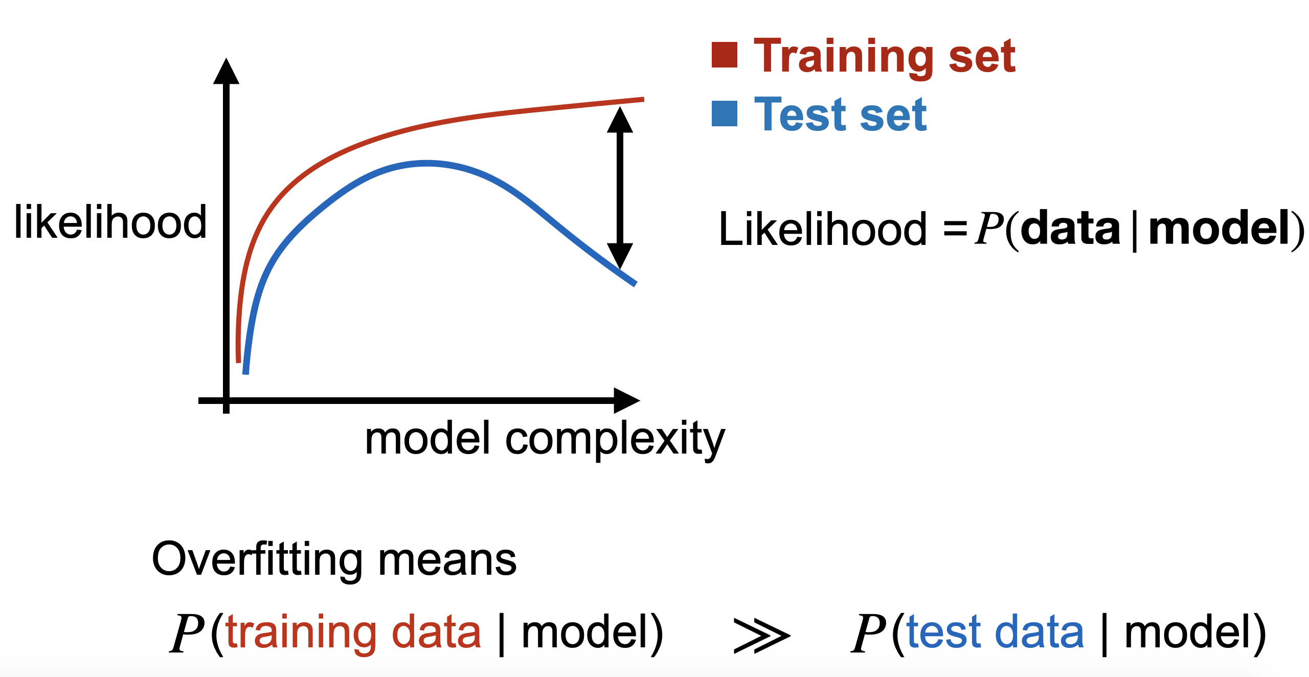
It is well understood that our models tend to do the same – deftly regurgitating their training data, yet struggling to generalize to unseen examples similar to the training data. Learning theory has nicely formalized this in the supervised setting. Our classification and regression models start to overfit when we observe a gap between training and (held-out) test prediction error, as in the above figure for the overly complex models.
This notion of overfitting relies on being able to measure prediction error or perhaps log likelihood of the labels, which is rarely a barrier in the supervised setting; supervised models generally output low dimensional, simple predictions. Such is not the case in the generative setting where we ask models to output original, high dimensional, complex entities like images or natural language. Here, we certainly lack any notion of prediction error and likelihoods are intractable for many of today’s generative models like VAEs and GANs: VAEs only provide a lower bound of the data likelihood, and GANs only leave us with their samples. This prevents us from simply measuring the gap between train and test accuracy/likelihood and calling it a day as we do with supervised models.
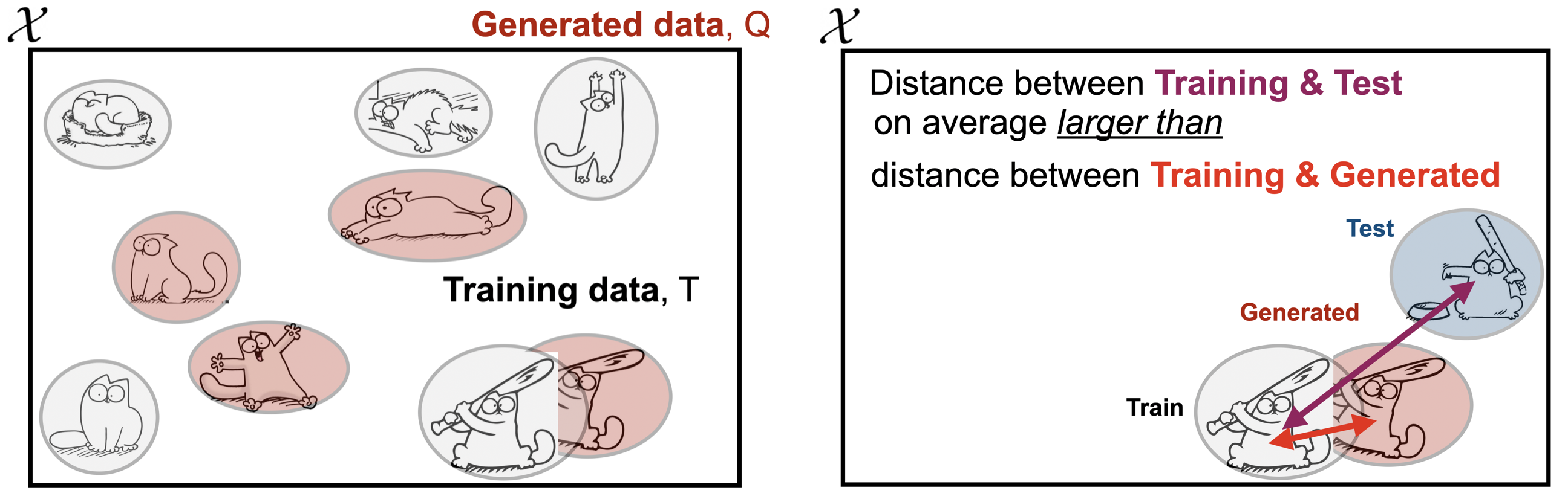
Instead, we evaluate generative models by comparing their generated samples with those of the true distribution, as in the following figure. Here, a two-sample test only uses a training sample and a generated sample. A three-sample test uses an additional held out test sample from the true distribution.
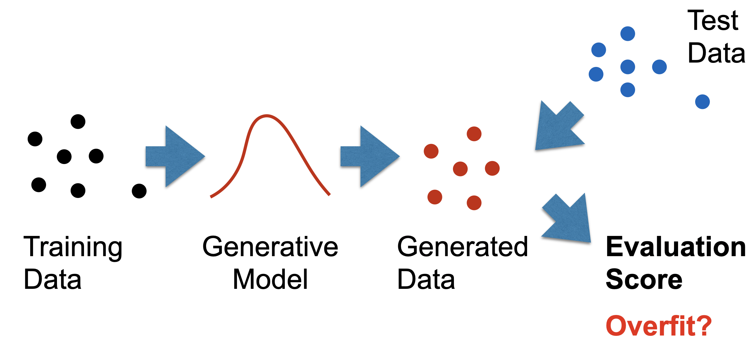
This practice is well established by existing two-sample generative model tests like the Frechet Inception Distance, Kernel MMD, and Precision & Recall test. But in absence of ground truth labels, what exactly are we testing for? We argue that unlike supervised models, generative models exhibit two varieties of overfitting: over-representation and data-copying.
Data-copying vs. Over-representation
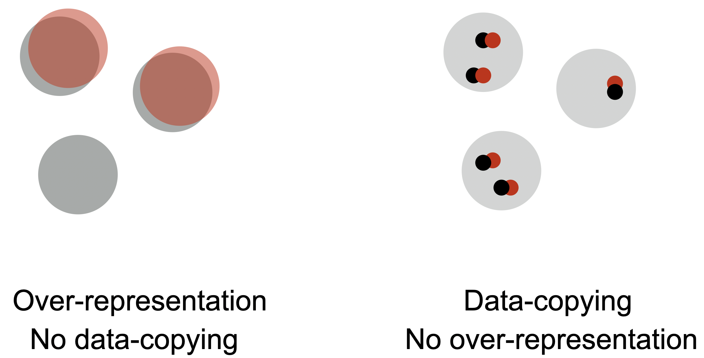
Most generative model tests like those listed above check for over-representation: the tendency of a model to over-emphasize certain regions of the instance space by assigning more probability mass there than it should. Consider a data distribution $P$ over an instance space $\mathcal{X}$ of cat cartoons. Region $\mathcal{C} \subset \mathcal{X}$ specifically contains cartoons of cats with bats. Using training set $T \sim P$, we train a generative model $Q$ from which we draw a sample $Q_m \sim Q$.
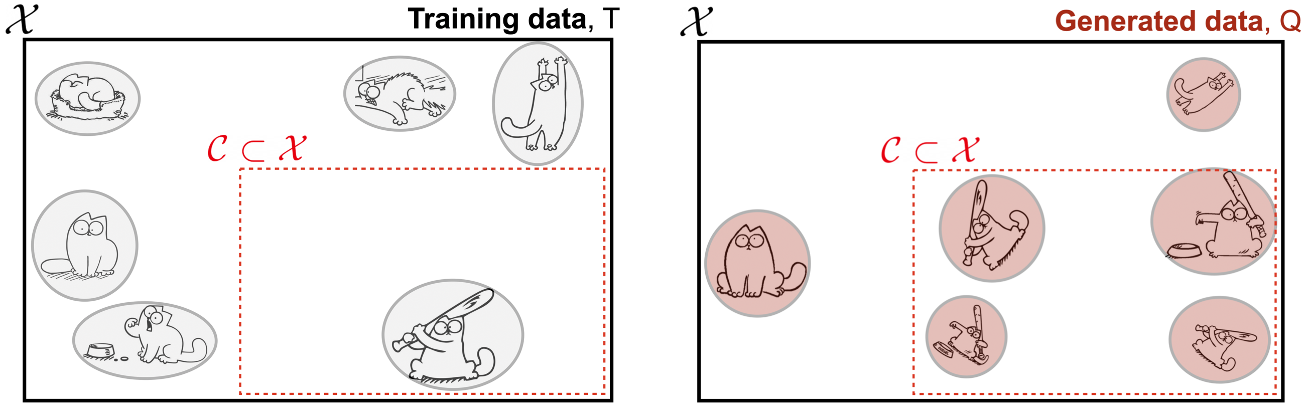
Evidently, the model $Q$ really likes region $\mathcal{C}$, generating an undue share of cats with bats. More formally, we say $Q$ is over-representing some region $\mathcal{C}$ when
\[ \Pr_{x \sim Q}[x \in \mathcal{C}] \gg \Pr_{x \sim P}[x \in \mathcal{C}] \]
This can be measured with a simple two-sample hypothesis test, as was done in Richardson & Weiss’s 2018 paper demonstrating the efficacy of Gaussian mixture models in high dimension.
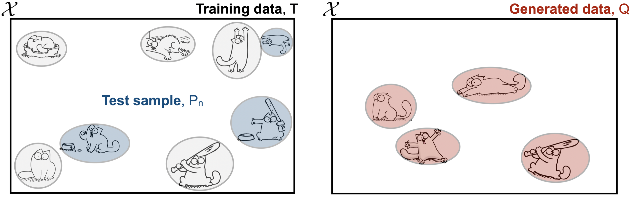
Data-copying, on the other hand, occurs when $Q$ produces samples that are closer to training set $T$ than they should be. To test for this, we equip ourselves with a held-out test sample $P_n \sim P$ in addition to some distance metric $d(x,T)$ that measures proximity to the training set of any $x \in \mathcal{X}$. We then say that $Q$ is data-copying training set $T$ when examples $x \sim Q$ are on average closer to $T$ than are $x \sim P$.
We define proximity to training set $d(x,T)$ to be the distance between $x$ and its nearest neighbor in $T$ according to some metric $d_\mathcal{X}:\mathcal{X} \times \mathcal{X} \rightarrow \mathbb{R}$. Specifically
\[ d(x,T) = \min_{t \in T}d_\mathcal{X}(x,t) \]
At a first glance, the generated samples in the above figure look perfectly fine, representing the different regions nicely. But taken alongside its training and test sets, we see that it has effectively copied the cat with bat in the lower right corner (for visualization, we let Euclidean distance $d_\mathcal{X}$ be a proxy for similarity).
More formally, $Q$ is data-copying $T$ in some region $\mathcal{C} \subset \mathcal{X}$ when
\[ \Pr_{x \sim Q, z \sim P}[d(x,T) < d(z,T) \mid x,z \in \mathcal{C}] \gg \frac{1}{2}\]
The key takeaway here is that data-copying and over-representation are orthogonal failure modes of generative models. A model that exhibits over-representation may or may not data-copy and vice versa. As such, it is critical that we test for both failure modes when designing and training models.
Returning to my failed culinary ambitions, I tend to both data-copy recipes I’ve tried and over-represent certain types of cuisine. If you look at the ‘true distribution’ of recipes online, you will find that there is a tremendous diversity of cooking styles and cuisines. However, put in the unfortunate circumstance of having me cook for you, I will most likely produce some slight variation of a recipe I’ve recently tried. And, even though I have attempted a number of Indian, Mexican, Italian, and French dishes, I tend to over-represent bland pastas and salads when left to my own devices. To cook truly original food, one must both be creative enough to go beyond the recipes they’ve seen and versatile enough to make a variety of cuisines. So, be sure to test for both data-copying and over-representation, and do not ask me to cook for you.
A Three-Sample Test for Data-Copying
Adding another test to one’s modeling pipeline is tedious. The good news is that data-copying can be tested with a single snappy three-sample hypothesis test. It is non-parametric, and concentrates nicely with both increasing test-set and generated samples.
As described in the previous section, we use a training sample $T \sim P$, a held-out test sample $P_n \sim P$, and a generated sample $Q_m \sim Q$. We additionally need some distance metric $d_\mathcal{X}(x,z)$. In practice, we choose $d_\mathcal{X}(x,z)$ to be the Euclidean distance between $x$ and $z$ after being embedded by $\phi$ into some lower-dimensional perceptual space: $d_\mathcal{X}(x,z) = \| \phi(x) - \phi(z) \|_2$. The use of such embeddings is common practice in testing generative models as exhibited by several existing over-representation tests like Frechet Inception Distance and Precision & Recall.
Following intuition, it is tempting to check for data-copying by simply differencing the expected distance to training set:
where, to reiterate, $d(x,T)$ is the distance $d_\mathcal{X}$ between $x$ and its nearest neighbor in $T$. This statistic — an expected distance — is a little too finicky: the variance is far out of our control, influenced by both the choice of distance metric and by outliers in both $P_n$ and $Q_m$. So, instead of probing for how much closer $Q$ is to $T$ than $P$ is, we probe for how often $Q$ is closer to $T$ than $P$ is:
This statistic — a probability — is closer to what we want to measure, and is more stable. It tells us how much more likely samples in $Q_m$ are to fall near samples in $T$ relative to the held out samples in $P_n$. If it is much less than a half, then significant data-copying is occurring. This statistic is much more robust to outliers and is lower variance. Additionally, by measuring a probability instead of an expected distance, the value of this statistic is interpretable. Regardless of the data domain or distance metric, less than half is overfit, half is good, and over half is underfit (in the sense that the generated samples are further from the training set than they should be). We are also able to show that this indicator statistic has nice concentration properties agnostic to the chosen distance metric.
It turns out that the above test is an instantiation of the Mann-Whitney hypothesis test, proposed in 1947, for which there are computationally efficient implementations in packages like SciPy. By $Z$-scoring the Mann-Whitney statistic, we normalize its mean to zero and variance to one. We call this statistic $Z_U$. As such, a generative model $Q$ with $Z_U \ll 0$ is heavily data-copying and a score $Z_U \gg 0$ is underfitting. Near 0 is ideal.
Handling Heterogeneity
An operative phrase that you may have noticed in the above definition of data-copying is “on average”. Is the generative model closer to the training data than it should be on average? This, unfortunately, is prone to false negatives. If $Z_U \ll 0$, then $Q$ is certainly data-copying in some region $\mathcal{C} \subset \mathcal{X}$. However, if $Z_U \geq 0$, it may still be excessively data-copying in one region and significantly underfitting in another, leading to a test score near 0.
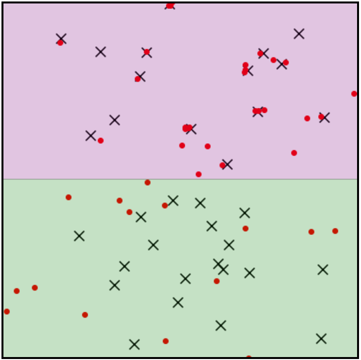
For example, let the $\times$’s denote training samples and the red dots denote generated samples. Even without observing a held-out test sample, it is clear that $Q$ is data-copying in pink region and underfitting in the green region. $Z_U$ will fall near 0, suggesting the model is performing well despite this highly undesirable behavior.
To prevent this misreading, we employ an algorithmic tool seen frequently in non-parametric testing: binning. Break the instance space into a partition $\Pi$ consisting of $k$ ‘bins’ or ‘cells’ $\pi \in \Pi$ and collect $Z_U^\pi$ each cell $\pi$.
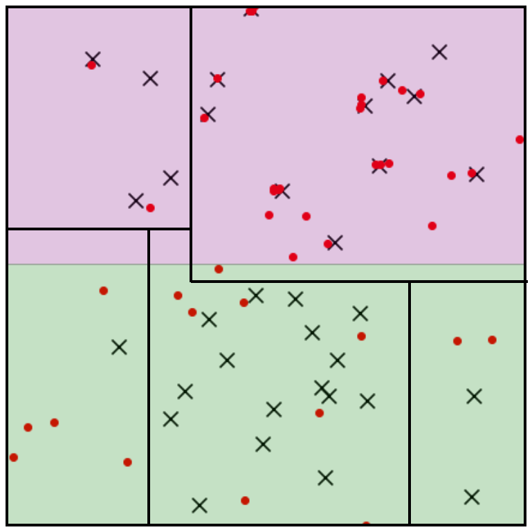
The statistic maintains its concentration properties within each cell. The more test and generated samples we have ($n$ and $m$), the more bins we can construct, and the more we can precisely pinpoint a model’s data-copying behavior. The ‘goodness’ of model’s fit is an inherently multidimensional entity, and it is informative to explore the range of $Z_U^\pi$ values seen in all cells $\pi \in \Pi$. Our experiments indicate that VAEs and GANs both tend to data-copy in some cells and underfit in others. However, to boil all this down into a single statistic for model comparisons, we simply take an average of the $Z_U^\pi$ values weighted by the number of test samples in the cell:
(In practice, we restrict ourselves to cells with a sufficient number of generated samples. See the paper.). Intuitively, this statistic tells us whether the model tends to data-copy in the regions most heavily emphasized by the true distribution. It does not tell us whether or not the model $Q$ data-copies somewhere.
Experiments: data-copying in the wild
Observing data-copying in VAEs and GANs indicates that the $C_T$ statistic above serves as an instructive tool for model selection. For a more methodical interrogation of the $C_T$ statistic and comparison with baseline tests, be sure to check out the paper.
To test how VAE complexity relates to data-copying, we train 20 VAEs on MNIST with increasing width as indicated by the latent dimension. For each model $Q$, we draw a sample of generated images $Q_m$, and compare with a held out test set $P_n$ to measure $C_T$. Our distance metric is given by the 64d latent space of an autoencoder we trained with a VGG perceptual loss produced by Zhang et al.. The purpose of this alternative latent space is to provide an embedding that both provides a perceptual distance between images and is independent of the VAE embeddings. For partitioning, we simply take the Voronoi cells induced by the $k$ centroids found by $k$-means run on the embedded training dataset.
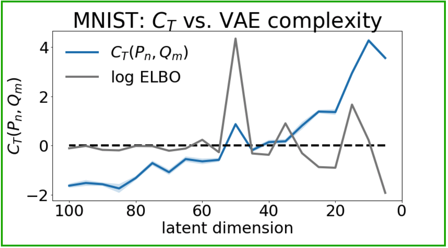
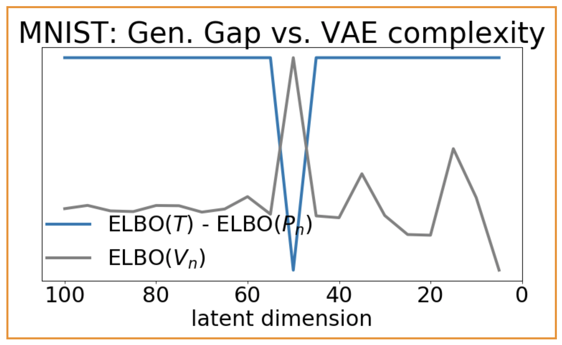
The data-copying $C_T$ statistic (left) captures overfitting in overly complex VAEs. The train/test gap in ELBO (right), meanwhile, does not.
Recall that $C_T \ll 0$ indicates data-copying and $C_T \gg 0$ indicates underfitting. We see (above, left) that overly complex models (towards the left of the plot) tend to copy their training set, and simple models (towards the right of the plot) tend to underfit, just as we might expect. Furthermore, $C_T = 0$ approximately coincides with the maximum ELBO, the VAE’s likelihood lower bound. For comparison, take the generalization gap of the VAEs’ ELBO on the training and test sets (above, right). The gap remains large for both overly complex models ($d > 50$) and simple models ($d < 50$). With the ELBO being a lower bound to the likelihood, it is difficult to interpret precisely why this happens. Regardless, it is clear that the ELBO gap is a compartively imprecise measure of overfitting.
While the VAEs exhibit increasing data-copying with model complexity on average, most of them have cells that are over- and underfit. Poking into the individual cells $\pi \in \Pi$, we can take a look at the difference between a $Z_U^\pi \ll 0$ cell and a $Z_U^\pi \gg 0$ cell:
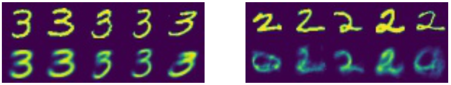
A VAE's datacopied (left) vs. underfit (right) cells of the MNIST instance space.
The two strips exhibit two regions of the same VAE. The bottom row of each shows individual generated samples from the cell, and the top row shows their training nearest neighbors. We immediately see that the data-copied region (left, $Z_U^\pi = -8.54$) practically produces blurry replicas of its training nearest neighbors, while the underfit region (right, $Z_U^\pi = +3.3)$ doesn’t appear to produce samples that look like any training image.
Extending these tests to a more complex and practical domain, we check the ImageNet-trained BigGAN model for data-copying. Being a conditional GAN that can output images of any single ImageNet 12 class, we condition on three separate classes and treat them as three separate models: Coffee, Soap Bubble, and Schooner. Here, it is not so simple to re-train GANs of varying degrees of complexity as we did before with VAEs. Instead, we modulate the model’s ‘trunction threshold’: a level beyond which all inputs are resampled. A larger truncation threshold allows for higher variance latent input, and thus higher variance outputs.
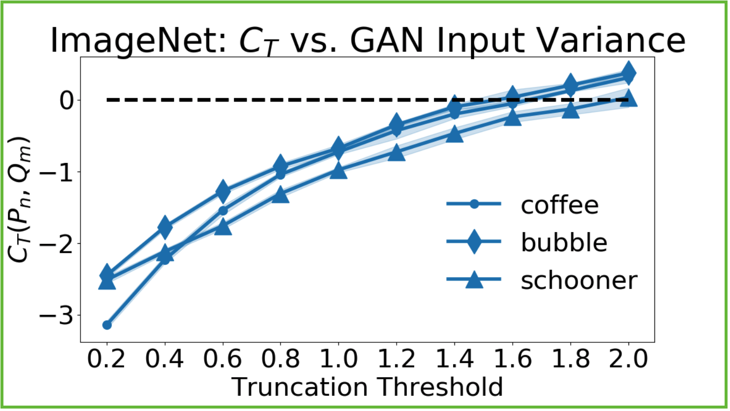
BigGan, an ImageNet12 conditional GAN, appears to significantly data-copy for all but its highest truncation levels, which are said to trade off between variety and fidelity.
Low truncation thresholds restrict the model to producing samples near the mode – those it is most confident in. However it appears that in all image classes, this also leads to significant data copying. Not only are the samples less diverse, but they hang closer to the training set than they should. This contrasts with the BigGAN authors’ suggestion that truncation level trades off between ‘variety and fidelity’. It appears that it might trade off between ‘copying and not copying’ the training set.
Again, even the least copying models with maximized truncation (=2) exhibit data-copying in some cells $\pi \in \Pi$:
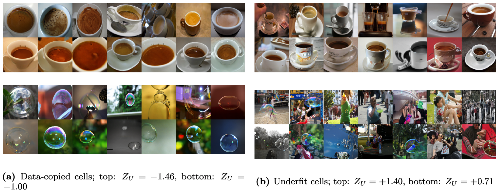
Examples from BigGan's data-copied (left) and underfit (right) cells of the 'coffee' (top) and 'soap bubble' (bottom) classes.
The left two strips show show data-copied cells of the coffee and bubble instance spaces (low $Z_U^\pi$), and right two strips show underfit cells (high $Z_U^\pi$). The bottom row of each strip shows a subset of generated images from that cell, and the top row training images from the cell. To show the diversity of the cell, these are not necessarily the generated samples’ training nearest neighbors as they were in the MNIST example.
We see that the data-copied cells on the left tend to confidently produce samples of one variety, that linger too closely to some specific examples it caught in the training set. In the coffee case, it is the teacup/saucer combination. In the bubble case, it is the single large suspended bubble with blurred background. Meanwhile, the slightly underfit cells on the right arguably perform better in a ‘generative’ sense. The samples, albeit slightly distorted, are more original. According to the inception space distance metric, they hug less closely to the training set.
Data-copying is a real failure mode of generative models
The moral of these experiments is that data-copying indeed occurs in contemporary generative models. This failure mode has significant consequences for user privacy and for model generalization. With that said, it is a failure mode not identified by most prominent generative model tests in the literature today.
-
Data-copying is orthogonal to over-representation; both should be tested when designing and training generative models.
-
Data-copying is straightforward to test efficiently when equipped with a decent distance metric.
-
Having identified this failure mode, it would be interesting to see modeling techniques that actively try to minimize data-copying in training.
So be sure to start probing your models for data-copying, and don’t be afraid to venture off-recipe every once in a while!
More Details
Check out our AISTATS paper on arxiv, and our data-copying test code on GitHub.