Adversarial Robustness Through Local Lipschitzness
Neural networks are very susceptible to adversarial examples, a.k.a., small perturbations of normal inputs that cause a classifier to output the wrong label. The standard defense against adversarial examples is Adversarial Training, which trains a classifier using adversarial examples close to training inputs. This improves test accuracy on adversarial examples, but it often lowers clean accuracy, sometimes by a lot.
Several recent papers investigate whether an accuracy-robustness trade-off is necessary. Some pessimistic work says that unfortunately this may be the case, possibly due to high-dimensionality or computational infeasibility.
If a trade-off is unavoidable, then we have a dilemma: should we aim for higher accuracy or robustness or somewhere in between? Our recent paper explores an optimistic perspective: we posit that robustness and accuracy should be attainable together for real image classification tasks.
The main idea is that we should use a locally smooth classifier, one that doesn’t change its value too quickly around the data. Let’s walk through some theory about why this is a good idea. Then, we will explore how to use this in practice.
The problem with natural training
The reason why we see a trade-off between robustness and accuracy is due to training methods. The best neural network optimization methods lead to functions that change very rapidly, as this allows the network to closely fit the data.
Since we care about robustness, we actually want to move as slowly as possible from class to class. This is especially true for separated data. Think about an image dataset. Cats look different than dogs, and pandas look different than gibbons. Quantitatively, different animals should be far apart (for example, in $\ell_{\infty}$ and $\ell_2$ distance). It follows that we should be able to classify them robustly. If we are very confident in our prediction, then as long as we don’t modify a true image too much, we should output the same, correct label.
So why do adversarial perturbations lead to a high error rate? This is a very active area of research, and there’s no easy answer. As a step towards a better understanding, we present theoretical results on achieving perfect accuracy and robustness by using a locally smooth function. We also explore how well this works in practice.
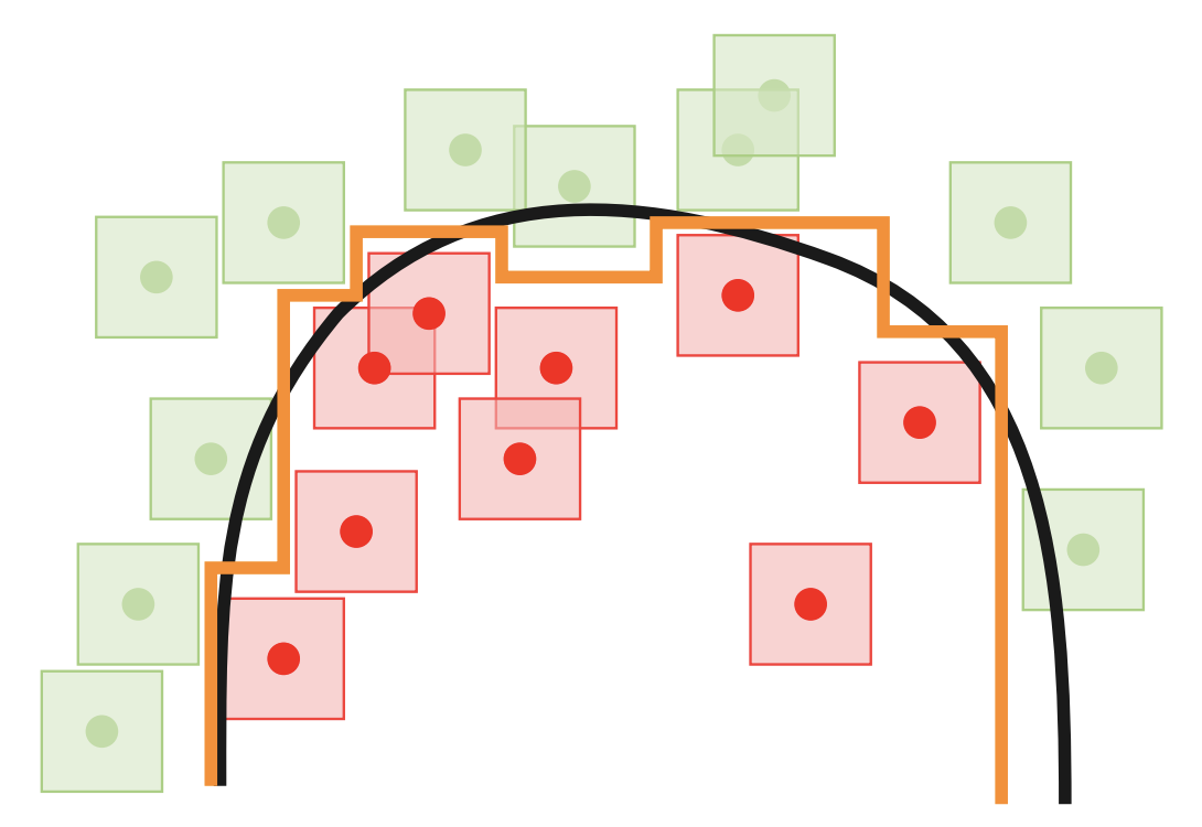
As a motivating example, consider a simple 2D binary classification dataset. The goal is to find a decision boundary that has 100% training accuracy without passing closely to any individual input. The orange curve in the following picture shows such a boundary. In contrast, the black curve comes very close to some data points. Even though both boundaries correctly classify all of the examples, the black curve is susceptible to adversarial examples, while the orange curve is not.
Perfect accuracy and robustness, at least in theory
We propose designing a classifier using the sign of a relatively smooth function. For separated data, this ensures that it’s impossible to change the label by slightly perturbing a true input. In other words, if the function value doesn’t change very quickly, then neither does the label.
More formally, we consider classifiers $g(x) = \mathsf{sign}(f(x))$, and we highlight the local Lipschitzness of $f$ as an important quantity. Simply put, the Lipschitz constant of a function measures how fast a function changes by dividing the difference between function values by the distance between inputs: $\frac{|f(x) - f(y)|}{d(x,y)}.$ Here $d(x,y)$ can be any metric. It is most common to use $d(x,y) = \|x - y\|$ for some norm on $\mathbb{R}^d$. Previous works (1, 2) shows that enforcing global Lipschitzness is too strict. Instead, we consider when $f$ is $L$-locally Lipschitz, which means that it changes slowly, at rate $L$, in a small neighborhood of radius $r$ around it.
Previous work by Hein and Andriushchenko has shown that local Lipschitzness indeed guarantees robustness. In fact, variants of Lipschitzness have been the main tool in certifying robustness with randomized smoothing as well. However, we are the first to identify a natural condition (data separation) that ensures both robustness and high test accuracy.
Our main theoretical result says that if the two classes are separated – in the sense that points from different classes are distance at least $2r$ apart, then there exists a $1/r$-locally Lipschitz function that is both robust to perturbations of distance $r$ and also 100% accurate.
For many real world datasets, the separation assumption in fact holds.
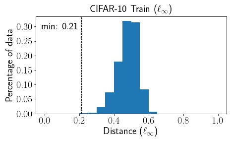
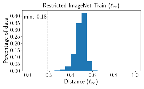
For example, consider the CIFAR-10 and Restricted ImageNet datasets (for the latter, we removed a handful of images that appeared twice with different labels). The figure shows the histogram of the $\ell_\infty$ distance of each training example to its closest differently-labeled example. From the figure we can see that the dataset is $0.21$ separated, indicating that there exists a solution that’s both robust and accurate with a perturbation distance up to $0.105$. Perhaps surprisingly, most work on adversarial examples considers small perturbations of size $0.031$ for CIFAR-10 and $0.005$ for Restricted ImageNet, which are both much less than the observed separation in these histograms.
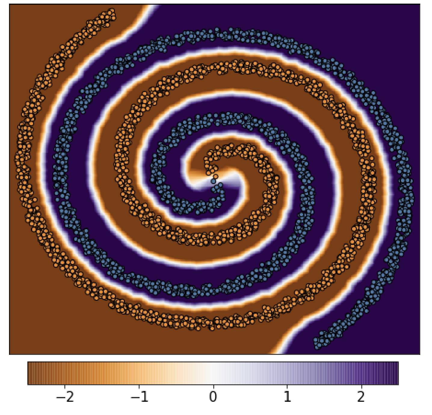
We basically use a scaled version of the 1-nearest neighbor classifier in the infinite sample limit. The proof just uses the data separation along with a few applications of the triangle inequality. The next figure shows our theorem in action on the Spiral dataset. The classifier $g(x) = \mathsf{sign}(f(x))$ has high adversarial and clean accuracy, while the small local Lipschitz constant ensures that it gradually changes near the decision boundaries.
Encouraging the smoothness of neural networks
Now that we’ve made a big deal of local Lipschitzness, and provided some theory to back it up, we want to see how well this holds up in practice. Two questions drive our experiments:
- Is local Lipschitzness correlated with robustness and accuracy in practice?
- Which training methods produce locally Lipschitz functions?
We also need to explain how we measure Lipschitzness on real data. For simplicity, we consider the average local Lipschitzness, computed using
\[ \frac{1}{n}\sum_{i=1}^n\max_{x_i’\in\mathsf{Ball}(x_i,\epsilon)}\frac{|f(x_i)-f(x_i’)|}{\|x_i-x_i’\|_\infty}. \]
The benefit is that we want the function to be smooth on average, even though there may be some outliers. One of the best methods for adversarial examples is TRADES, which encourages local Lipschitzness by minimizing the following loss function:
\[ \min_{f} \mathbb{E} \Big\{\mathcal{L}(f(X),Y)+\beta\max_{X’\in\mathsf{Ball}(X,\epsilon)} \mathcal{L}(f(X),f(X’))\Big\}. \]
TRADES is different than Adversarial Training (AT), which optimizes the following:
\[ \min_{f} \mathbb{E} \Big\{\max_{X’\in\mathsf{Ball}(X,\epsilon)}\mathcal{L}(f(X’),Y)\Big\}. \]
AT directly optimizes over adversarial examples, while TRADES encourages $f(X)$ and $f(X’)$ to be similar when $X$ and $X’$ are close to each other. The TRADES parameter $\beta$ controls the local smoothness (larger $\beta$ means a smaller Lipschitz constant).
We also consider two other plausible methods for achieving accuracy and robustness, along with local Lipschitzness: Local Linear Regularization (LLR) and Gradient Regularization (GR).
Comparing five different training methods
Here we provide experimental results for CIFAR-10 and Restricted ImageNet. See our paper for other datasets (MNIST and SVHN).
| CIFAR-10 | train accuracy | test accuracy | adv test accuracy | test lipschitz |
|---|---|---|---|---|
| Natural | 100.00 | 93.81 | 0.00 | 425.71 |
| GR | 94.90 | 80.74 | 21.32 | 28.53 |
| LLR | 100.00 | 91.44 | 22.05 | 94.68 |
| AT | 99.84 | 83.51 | 43.51 | 26.23 |
| TRADES($\beta$=1) | 99.76 | 84.96 | 43.66 | 28.01 |
| TRADES($\beta$=3) | 99.78 | 85.55 | 46.63 | 22.42 |
| TRADES($\beta$=6) | 98.93 | 84.46 | 48.58 | 13.05 |
| Restricted ImageNet | train accuracy | test accuracy | adv test accuracy | test lipschitz |
|---|---|---|---|---|
| Natural | 97.72 | 93.47 | 7.89 | 32228.51 |
| GR | 91.12 | 88.51 | 62.14 | 886.75 |
| LLR | 98.76 | 93.44 | 52.65 | 4795.66 |
| AT | 96.22 | 90.33 | 82.25 | 287.97 |
| TRADES($\beta$=1) | 97.39 | 92.27 | 79.90 | 2144.66 |
| TRADES($\beta$=3) | 95.74 | 90.75 | 82.28 | 396.67 |
| TRADES($\beta$=6) | 93.34 | 88.92 | 82.13 | 200.90 |
For both datasets, we see correlation between accuracy, Lipschitzness, and adversarial accuracy. For example, on CIFAR-10, we see that TRADES($\beta$=6) achieves the highest adversarial test accuracy (48.58), and also the lowest Lipschitz constant (13.05). TRADES may not always perform better than AT, but it seems like a very effective method to produce classifiers with small local Lipschitz constants. One issue is that the training accuracy isn’t as high as it could be, and there are some issues with tuning the methods to prevent underfitting. In general, we focus on understanding the role of Lipschitzness.
Natural training has the lowest adversarial accuracy, and also the higher Lipschitz constant. GR has a fairly low training accuracy (possibly due to underfitting). For LLR, AT, and TRADES, we see that smoother classifiers have higher adversarial test accuracy as well. However, this is only true up to some point. Increased local Lipschitzness helps, but with very high local Lipschitzness, the neural networks start underfitting which leads to loss in accuracy, for example, with TRADES($\beta$=6).
Robustness requires some local Lipschitzness
Our experimental results provide many insights into the role that Lipschitzness plays in classifier accuracy and robustness.
-
A clear takeaway is that very high Lipschitz constants imply that the classifier is vulnerable to adversarial examples. We see this most clearly with natural training, but it is also evidenced by GR and LLR.
-
For both CIFAR and Restricted ImageNet, the experiments show that minimizing the Lipschitzness goes hand-in-hand with maximizing the adversarial accuracy. This highlights that Lipschitzness is just as important as training with adversarial examples when it comes to improving the adversarial robustness.
-
TRADES always leads to significantly smaller Lipschitz constants than most methods, and the smoothness increases with the TRADES parameter $\beta$. However, the correlation between smoothness and robustness suffers from diminishing returns. It is not optimal to minimize the Lipschitzness as much as possible.
-
The main downside of AT and TRADES is that the clean accuracy suffers. This issue may not be inherent to robustness, but rather it may be possible to achieve the best of both worlds. For example, LLR is consistently more robust than natural training, while simultaneously achieving state-of-the-art clean test accuracy. This leaves open the possibility of combining the benefits of both LLR and AT/TRADES into a classifier that does well across the board. This is the main future work!
More Details
See our paper on arxiv or our repository.