DYffusion: A Dynamics-informed Diffusion Model for Spatiotemporal Forecasting
We introduce a novel diffusion model-based framework, DYffusion, for large-scale probabilistic forecasting. We propose to couple the diffusion steps with the physical timesteps of the data, leading to temporal forward and reverse processes that we represent through an interpolator and a forecaster network, respectively. DYffusion is faster than standard diffusion models during sampling, has low memory needs, and effectively addresses the challenges of generating stable, accurate and probabilistic rollout forecasts.
Introduction
Obtaining accurate and reliable probabilistic forecasts has a wide range of applications from
climate simulations and fluid dynamics to financial markets and epidemiology.
Often, accurate long-range probabilistic forecasts are particularly challenging to obtain
Common approaches for large-scale spatiotemporal problems tend to be deterministic and autoregressive. Thus, they are often unable to capture the inherent uncertainty in the data, produce unphysical predictions, and are prone to error accumulation for long-range forecasts.
Diffusion models have shown great success for natural image and video generation. However, diffusion models have been primarily designed for static data and are expensive to train and to sample from. We study how we can efficiently leverage them for large-scale spatiotemporal problems and explicitly incorporate the temporality of the data into the diffusion model.
Our Key Idea
We introduce a solution for these issues by designing a temporal diffusion model, DYffusion.
Following the “generalized diffusion model” framework
Notation & Background
Problem setup
We study the problem of probabilistic spatiotemporal forecasting using a dataset consisting of a time series of snapshots \(\mathbf{x}_t \in \mathcal{X}\). We focus on the task of forecasting a sequence of \(h\) snapshots from a single initial condition. That is, we aim to train a model to learn \(P(\mathbf{x}_{t+1:t+h} \,|\, \mathbf{x}_t)\) . Note that during evaluation, we may evaluate the model on a larger horizon \(H>h\) by running the model autoregressively.
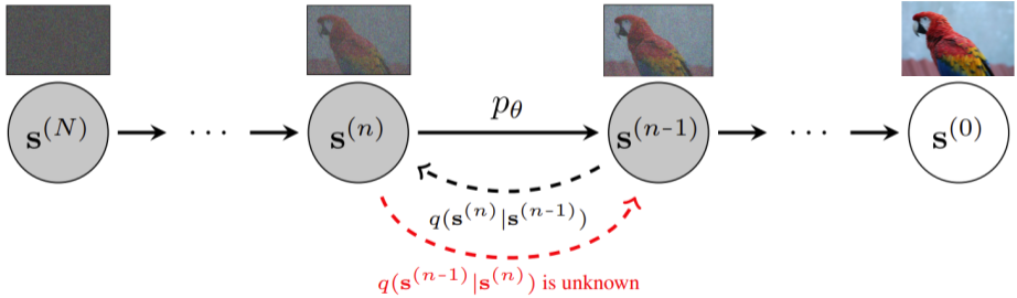
Standard diffusion models
Diffusion models iteratively transform data between an initial distribution
and the target distribution over multiple diffusion steps
DYffusion: Dynamics-informed Diffusion Model
The key innovation of our framework, DYffusion, is a reimagining of the diffusion processes to more naturally model
spatiotemporal sequences, \(\mathbf{x}_{t:t+h}\).
Specifically, we design the reverse (forward) process to step forward (backward) in time
so that our diffusion model emulates the temporal dynamics in
the data
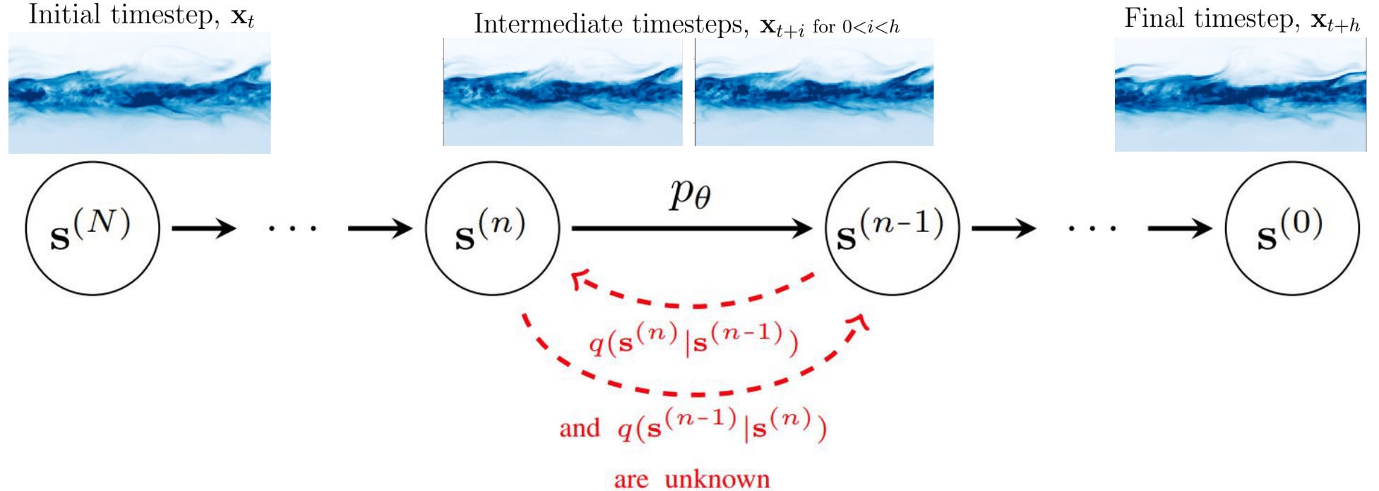
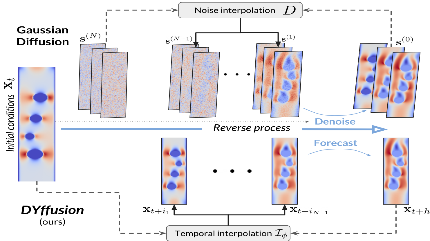
Implementation-wise, we replace the standard denoising network, \(R_\theta\), with a deterministic forecaster network, \(F_\theta\). Because we do not have a closed-form expression for the forward process, we also need to learn it from data by replacing the standard forward process operator, \(D\), with a stochastic interpolator network \(\mathcal{I}_\phi\). Intermediate steps in DYffusion’s reverse process can be reused as forecasts for actual timesteps. Another benefit of our approach is that the reverse process is initialized with the initial conditions of the dynamics and operates in observation space at all times. In contrast, a standard diffusion model is designed for unconditional generation, and reversing from white noise requires more diffusion steps.
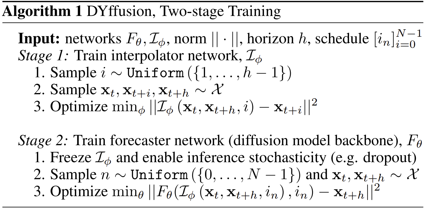
Training DYffusion
We propose to learn the forward and reverse process in two separate stages:
Temporal interpolation as a forward process
To learn our proposed temporal forward process, we train a time-conditioned network \(\mathcal{I}_\phi\) to interpolate between snapshots of data. Given a horizon \(h\), we train the interpolator net so that \(\mathcal{I}_\phi(\mathbf{x}_t, \mathbf{x}_{t+h}, i) \approx \mathbf{x}_{t+i}\) for \(i \in \{1, \ldots, h-1\}\) using the objective:
\[\begin{equation} \min_\phi \mathbb{E}_{i \sim \mathcal{U}[\![1, h-1]\!], \mathbf{x}_{t, t+i, t+h} \sim \mathcal{X}} \left[\| \mathcal{I}_\phi(\mathbf{x}_t, \mathbf{x}_{t+h}, i) - \mathbf{x}_{t+i} \|^2 \right]. \label{eq:interpolation} \end{equation}\]Interpolation is an easier task than forecasting, and we can use the resulting interpolator
for temporal super-resolution during inference to interpolate beyond the temporal resolution of the data.
That is, the time input can be continuous, with \(i \in (0, h-1)\).
It is crucial for the interpolator, \(\mathcal{I}_\phi\),
to produce stochastic outputs within DYffusion so that its forward process is stochastic, and it can generate probabilistic forecasts at inference time.
We enable this using Monte Carlo dropout
Forecasting as a reverse process
In the second stage, we train a forecaster network \(F_\theta\) to forecast \(\mathbf{x}_{t+h}\) such that \(F_\theta(\mathcal{I}_\phi(\mathbf{x}_{t}, \mathbf{x}_{t+h}, i \vert \xi), i)\approx \mathbf{x}_{t+h}\) for \(i \in S =[i_n]_{n=0}^{N-1}\), where \(S\) denotes a schedule coupling the diffusion step to the interpolation timestep. The interpolator network, \(\mathcal{I}\), is frozen with inference stochasticity enabled, represented by the random variable \(\xi\). In our experiments, \(\xi\) stands for the randomly dropped out weights of the neural network and is omitted henceforth for clarity. Specifically, we seek to optimize the objective
\[\begin{equation} \min_\theta \mathbb{E}_{n \sim \mathcal{U}[\![0, N-1]\!], \mathbf{x}_{t, t+h}\sim \mathcal{X}} \left[\| F_\theta(\mathcal{I}_\phi(\mathbf{x}_{t}, \mathbf{x}_{t+h}, i_n \vert \xi), i_n) - \mathbf{x}_{t+h} \|^2 \right]. \label{eq:forecaster} \end{equation}\]To include the setting where \(F_\theta\) learns to forecast the initial conditions, we define \(i_0 := 0\) and \(\mathcal{I}_\phi(\mathbf{x}_{t}, \cdot, i_0) := \mathbf{x}_t\). In the simplest case, the forecaster net is supervised by all timesteps given by the temporal resolution of the training data. That is, \(N=h\) and \(S = [j]_{j=0}^{h-1}\). Generally, the schedule should satisfy \(0 = i_0 < i_n < i_m < h\) for \(0 < n < m \leq N-1\).
Sampling from DYffusion
Our above design for the forward and reverse processes of DYffusion, implies the following generative process: \(\begin{equation} p_\theta(\mathbf{s}^{(n+1)} | \mathbf{s}^{(n)}, \mathbf{x}_t) = \begin{cases} F_\theta(\mathbf{s}^{(n)}, i_{n}) & \text{if} \ n = N-1 \\ \mathcal{I}_\phi(\mathbf{x}_t, F_\theta(\mathbf{s}^{(n)}, i_n), i_{n+1}) & \text{otherwise,} \end{cases} \label{eq:new-reverse} \end{equation}\)
where \(\mathbf{s}^{(0)}=\mathbf{x}_t\) and \(\mathbf{s}^{(n)}\approx\mathbf{x}_{t+i_n}\) correspond to the initial conditions and predictions of intermediate steps, respectively. In our formulations, we reverse the diffusion step indexing to align with the temporal indexing of the data. That is, \(n=0\) refers to the start of the reverse process, while \(n=N\) refers to the final output of the reverse process with \(\mathbf{s}^{(N)}\approx\mathbf{x}_{t+h}\). Our reverse process steps forward in time, in contrast to the mapping from noise to data in standard diffusion models. As a result, DYffusion should require fewer diffusion steps and data.
DYffusion follows the generalized diffusion model framework.
Thus, we can use existing diffusion model sampling methods for inference.
In our experiments, we adapt the sampling algorithm from
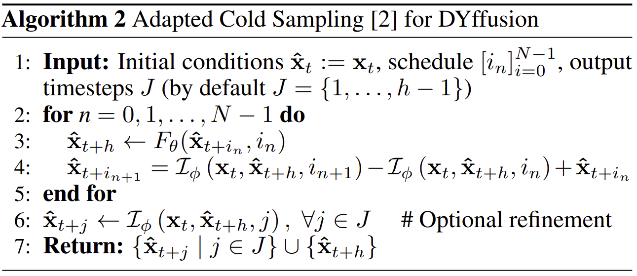
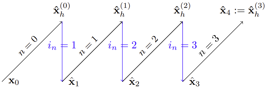
During the sampling process, our method essentially alternates between forecasting and interpolation, as illustrated in the figure below. \(R_\theta\) always predicts the last timestep, \(\mathbf{x}_{t+h}\), but iteratively improves those forecasts as the reverse process comes closer in time to \(t+h\). This is analogous to the iterative denoising of the “clean” data in standard diffusion models. This motivates line 6 of Alg. 2, where the final forecast of \(\mathbf{x}_{t+h}\) can be used to fine-tune intermediate predictions or to increase the temporal resolution of the forecast.
Memory footprint
During training, DYffusion only requires \(\mathbf{x}_t\) and \(\mathbf{x}_{t+h}\) (plus \(\mathbf{x}_{t+i}\) during the first interpolation stage),
resulting in a constant memory footprint as a function of \(h\).
In contrast, direct multi-step prediction models including video diffusion models or (autoregressive) multi-step loss approaches require
\(\mathbf{x}_{t:t+h}\) to compute the loss.
This means that these models must fit \(h+1\) timesteps of data into memory (and may need to compute gradients recursively through them),
which scales poorly with the training horizon \(h\).
Therefore, many are limited to predicting a small number of frames or snapshots.
For example, our main video diffusion model baseline, MCVD, trains on a maximum of 5 video frames due to GPU memory constraints
Experimental Setup
Datasets
We evaluate our method and baselines on three different datasets:
- Sea Surface Temperatures (SST): a new dataset based on NOAA OISSTv2
, which comes at a daily time-scale. Similarly to , we train our models on regional patches which increases the available data Here, we choose 11 boxes of $60$ latitude $\times 60$ longitude resolution in the eastern tropical Pacific Ocean. Unlike the data based on the NEMO dataset in . We train, validate, and test all models for the years 1982-2019, 2020, and 2021, respectively., we choose OISSTv2 as our SST dataset because it contains more data (although it has a lower spatial resolution of $1/4^\circ$ compared to $1/12^\circ$ of NEMO). - Navier-Stokes flow benchmark dataset from
, which consists of a \(221\times42\) grid. Each trajectory contains four randomly generated circular obstacles that block the flow. The channels consist of the \(x\) and \(y\) velocities as well as a pressure field and the viscosity is \(1e\text{-}3\). Boundary conditions and obstacle masks are given as additional inputs to all models. - Spring Mesh benchmark dataset from
. It represents a \(10\times10\) grid of particles connected by springs, each with mass 1. The channels consist of two position and momentum fields each.
We follow the official train, validation, and test splits from
Baselines
We compare our method against both direct applications of standard diffusion models to dynamics forecasting and methods to ensemble the “barebone” backbone network of each dataset. The network operating in “barebone” form means that there is no involvement of diffusion. We use the following baselines:
- DDPM
: We train it as a multi-step (video-like problem) conditional diffusion model. - MCVD
: A state-of-the-art conditional video diffusion model We train MCVD in "concat" mode, which in their experiments performed best. . - Dropout
: Ensemble multi-step forecasting of the barebone backbone network based on enabling dropout at inference time. - Perturbation
: Ensemble multi-step forecasting with the barebone backbone network based on random perturbations of the initial conditions with a fixed variance. - Official deterministic baselines from
for the Navier-Stokes and spring mesh datasets Due to their deterministic nature, we exclude these baselines from our main probabilistic benchmarks. .
MCVD and the multi-step DDPM predict the timesteps \(\mathbf{x}_{t+1:t+h}\) based on \(\mathbf{x}_{t}\).
The barebone backbone network baselines are time-conditioned forecasters trained on the multi-step objective
\(\mathbb{E}_{i \sim \mathcal{U}[\![1, h]\!], \mathbf{x}_{t, t+i}\sim \mathcal{X}}
\| F_\theta(\mathbf{x}_{t}, i) - \mathbf{x}_{t+i}\|^2\)
from scratch
Neural network architectures
For a given dataset, we use the same backbone architecture for all baselines as well as for both the interpolation and forecaster networks in DYffusion.
For the SST dataset, we use a popular UNet architecture designed for diffusion models.
For the Navier-Stokes and spring mesh datasets, we use the UNet and CNN from the original benchmark paper
Evaluation metrics
We evaluate the models by generating an M-member ensemble (i.e. M samples are drawn per batch element), where
we use M=20 for validation and M=50 for testing.
As metrics, we use the Continuous Ranked Probability Score (CRPS)
Results
Quantitative results
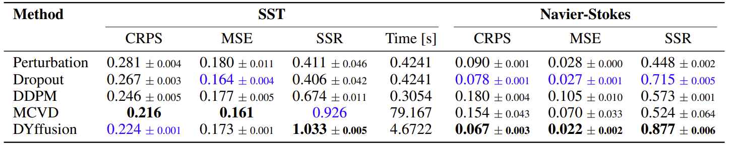
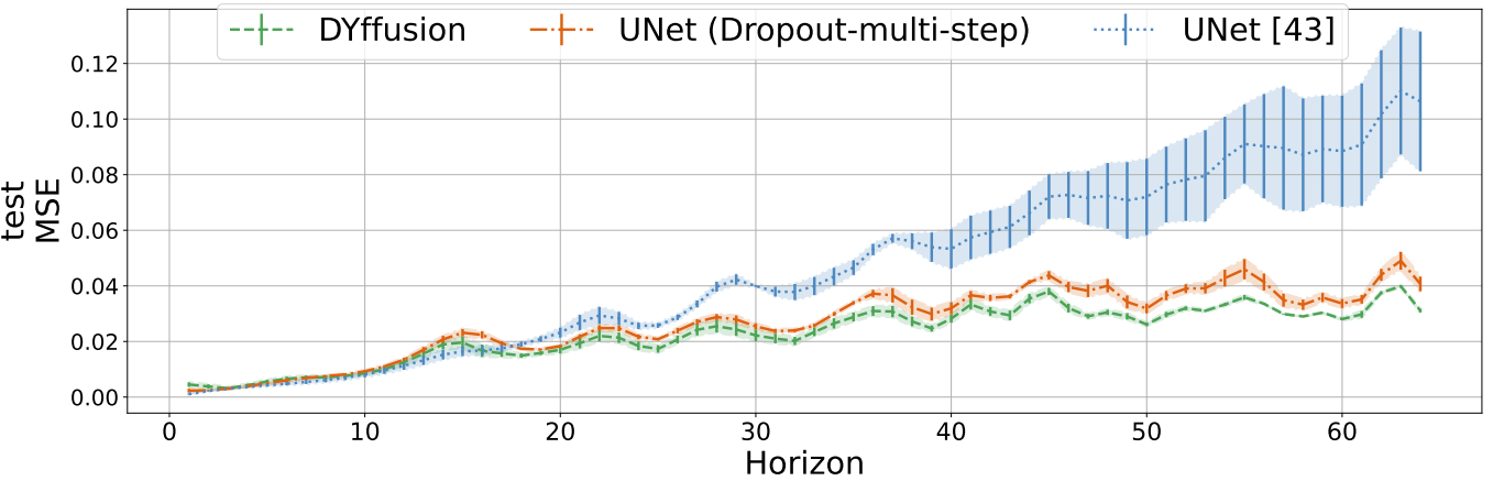
We present the time-averaged metrics for the SST and Navier-Stokes dataset in the table below. DYffusion performs best on the Navier-Stokes dataset, while coming in a close second on the SST dataset after MCVD, in terms of CRPS. Since MCVD uses 1000 diffusion steps, it is slower to sample from at inference time than from DYffusion, which is trained with at most 35 diffusion steps. The DDPM model for the SST dataset is fairly efficient because it only uses 5 diffusion steps but lags in terms of performance.
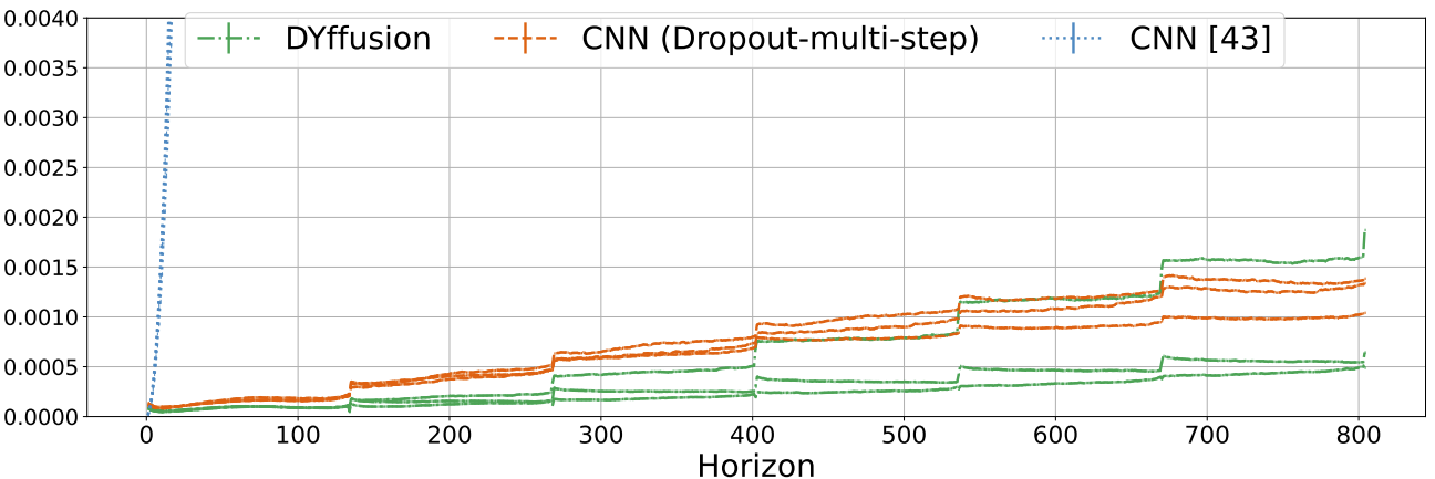
Thanks to the dynamics-informed and memory-efficient nature of DYffusion, we can scale our framework to long horizons. On the spring mesh dataset, we train with a horizon of 134 and evaluate the models on trajectories of 804 time steps. Our method beats the Dropout baseline, with a larger margin on the out-of-distribution test dataset. Despite several attempts with varying hyperparameter configurations neither the DDPM nor the MCVD diffusion model converged on this dataset.
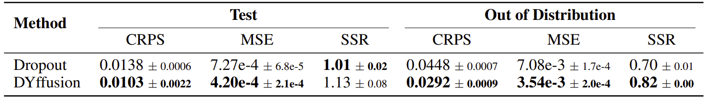
The reported MSE scores above, using the same CNN architecture,
are significantly better than the ones reported for the official CNN baselines in Fig. 8 of
Qualitative results
Long-range forecasts of ML models often suffer from blurriness or might even diverge when using autoregressive models. In the video below, we show a complete Navier-Stokes test trajectory forecasted by DYffusion and the best baseline, Dropout, as well as the corresponding ground truth. Our method can reproduce the true dynamics over the full trajectory and does so better than the baseline, especially for fine-scale patterns such as the tails of the flow after the right-most obstacle.
Temporal super-resolution and sample variability
Motivated by the continuous-time nature of DYffusion, we aim to study in this experiment whether it is possible to forecast skillfully beyond the resolution given by the data. Here, we forecast the same Navier-Stokes trajectory shown in the video above but at \(8\times\) resolution. That is, DYffusion forecasts 512 timesteps instead of 64 in total. This behavior can be achieved by either changing the sampling trajectory \([i_n]_{n=0}^{N-1}\) or by including additional output timesteps, \(J\), for the refinement step of line 6 in Alg. 2. In the video below, we choose to do the latter and find the 5 sampled forecasts to be visibly pleasing and temporally consistent with the ground truth.
Note that we hope that our probabilistic forecasting model can capture any of the possible, uncertain futures instead of forecasting their mean, as a deterministic model would do. As a result, some long-term rollout samples are expected to deviate from the ground truth. For example, see the velocity at t=3.70 in the video above. It is reassuring that DYffusion’s samples show sufficient variation, but also cover the ground truth quite well (sample 1). This advantage is also reflected quantitatively in the spread-skill ratio (SSR) metric, where DYffusion consistently reached values close to 1.
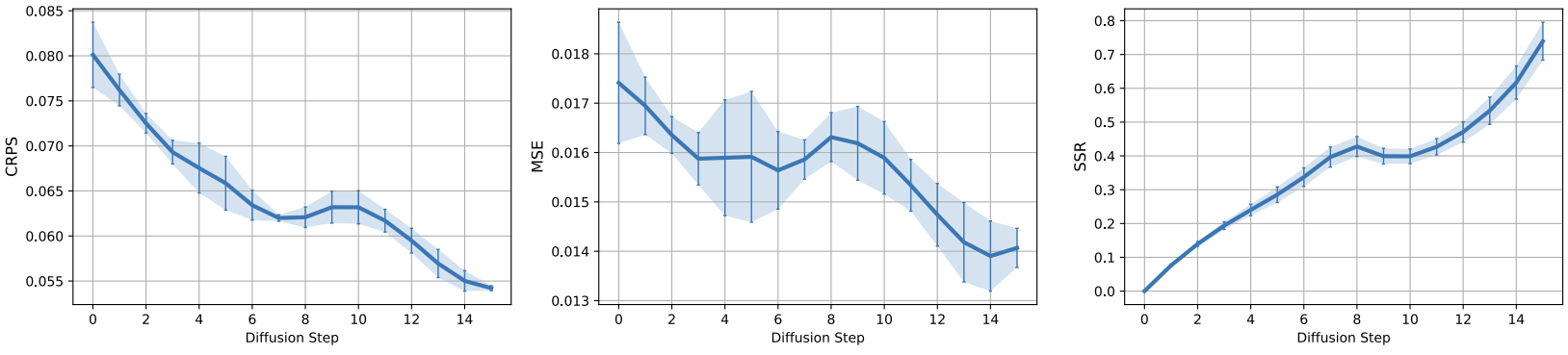
Iterative refinement of forecasts
DYffusion’s forecaster network repeatedly predicts the same timestep, \(t+h\), during sampling. Thus, we need to verify that these forecasts, \(\hat{\mathbf{x}}_{t+h} = F_\theta(\mathbf{x}_{t+i_n}, i_n)\), tend to improve throughout the course of the reverse process, i.e. as \(n\rightarrow N\) and \(\mathbf{x}_{t+i_n}\rightarrow\mathbf{x}_{t+h}\). Below we show that this is indeed the case for the Navier-Stokes dataset. Generally, we find that this observation tends to hold especially for the probabilistic metrics, CRPS and SSR, while the trend is less clear for the MSE across all datasets (see Fig. 7 of our paper).
Conclusion
DYffusion is the first diffusion model that relies on task-informed forward and reverse processes. Other existing diffusion models, albeit more general, use data corruption-based processes. Thus, our work provides a new perspective on designing a capable diffusion model, and we hope that it will lead to a whole family of task-informed diffusion models.
If you have any application that you think could benefit from DYffusion, or build on top of it, we would love to hear from you!
For more details, please check out our NeurIPS 2023 paper, and our code on GitHub.