Adversarial Robustness for Non-Parametric Classifiers
In a previous post, we discussed the relationship between accuracy and robustness for separated data. A classifier trained on $r$-separated data can be both accurate and robust with radius $r.$ What if the data are not $r$-separated? In our recent paper, we look at how to deal with this case.
Many datasets with natural data like images or audio are $r$-separated [1]. In contrast, datasets with artificially-extracted features are often not. Non-parametric methods like nearest neighbors, random forest, etc. perform well on these kind of datasets. In this post, we focus on the discussion of non-parametric methods on non-$r$-separated datasets.
We first present a defense algorithm – adversarial pruning – that can increase the robustness of many non-parametric methods. Then we dive into how adversarial pruning deals with non-$r$-separated data. Finally, we present a generic attack algorithm that works well across many non-parametric methods and use it to evaluate adversarial pruning.
Defense
Let us start by visualizing the decision boundaries of a $1$-nearest neighbor ($1$-NN) and a random forest (RF) classifier on a toy dataset.
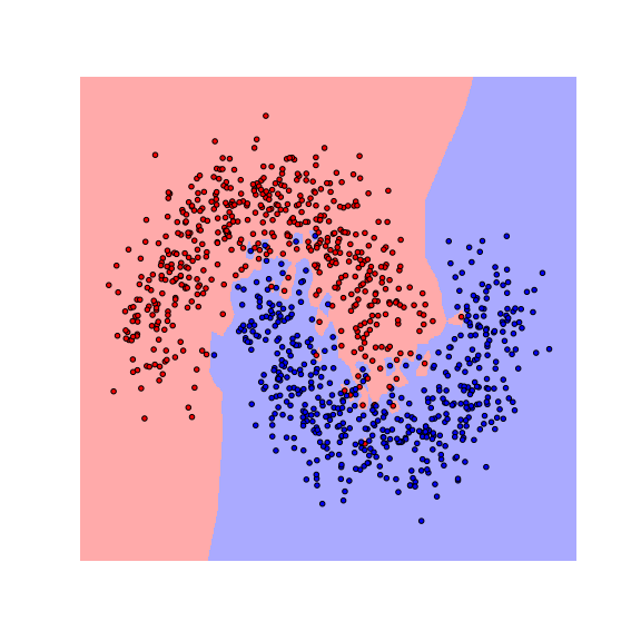
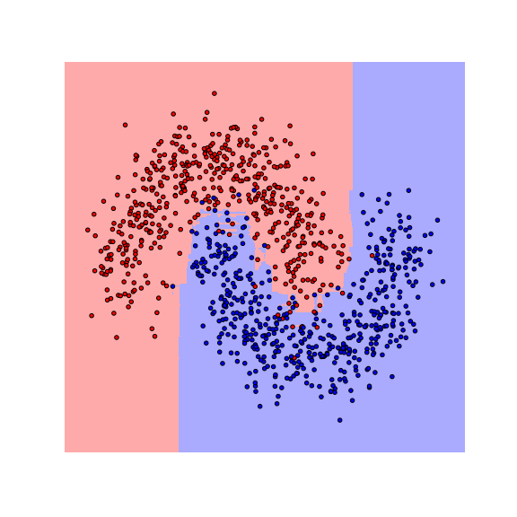
We see that the decision boundaries are highly non-smooth, and lie close to many data points, resulting in a non-robust classifier. This is caused by the fact that many differently-labeled examples are near each other. Next, let us consider a modified dataset in which the red and blue examples are more separated.
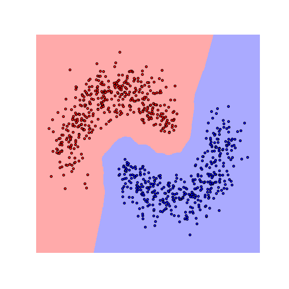

Notice that the boundaries become smoother as examples move further away from the boundaries. This makes the classifier more robust as the predicted label stays the same if data are perturbed a little.
Adversarial Pruning
From these figures, we can see that these non-parametric methods are more robust when data are better separated. Given a dataset, to make it more separated, we need to remove examples. To preserve information in the dataset, we do not want to remove too many examples. We design our defense algorithm to minimally remove examples from the dataset so that differently-labeled examples are well-separated from each other. After this modification, we can train a non-parametric classifier on it. We call this defense algorithm adversarial pruning (AP).
More formally, given a robustness radius $r$ and a training set $\mathcal{S}$, AP computes a maximum subset $\mathcal{S}^{AP} \subseteq \mathcal{S}$ such that differently-labeled examples in $\mathcal{S}^{AP}$ have distance at least $r$. We show that known graph algorithms can be used to efficiently compute $\mathcal{S}^{AP}$. We build a graph $G=(V, E)$ as follows. First, each training example is a vertex in the graph. We connect pairs of differently-labeled examples (vertices) $\mathbf{x}$ and $\mathbf{x}’$ with an edge whenever $|\mathbf{x} − \mathbf{x}’| \leq 2r$. Then, computing $\mathcal{S}^{AP}$ is reduced to removing as few examples as possible so that no more edges remain. This is equivalent to solving the minimum vertex cover problem. When dealing with binary classification problem, the graph $G$ is bipartite and standard algorithms like the Hopcroft–Karp algorithm can be used to solve this problem. With multi-class classification, minimum vertex cover is NP Hard in general, and approximation algorithms have to be applied.
Theoretical Justification
It happens that Adversarial Pruning has a nice theoretical interpretation - we can show that it can be interpreted as a finite sample approximation to the optimally robust and accurate classifier. To understand this, first, let us try to understand what the goal of robust classification is. We assume the data is sampled from a distribution $\mu$ on $\mathcal{X} \times [C]$, where $\mathcal{X}$ is the feature space and $C$ is the number of classes. Normally, the ultimate limit of accurate classification is the Bayes optimal classifier which maximizes the accuracy on the underlying data distribution. But the Bayes optimal may not be very robust.
Let us look at the figure below. The blue curve is the decision boundary of the Bayes optimal classifier. We see that this blue curve is close to the data distribution and thus not the most robust. An alternative decision boundary is the black curve, which is further away from the distribution while still being accurate.
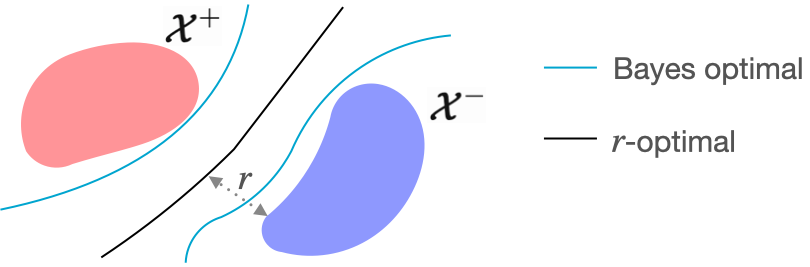
We define the astuteness of a classifier as its accuracy on examples where it is robust with radius $r$. The objective of a robust classifier is to maximize the astuteness under $\mu$, which is the probability that the classifier is both $r$-robust and accurate for a new sample $(\mathbf{x}, y)$ [1, 2].
Next, we present the $r$-optimal classifier that achieves optimal astuteness. By comparing it with the classic Bayes optimal classifier, which achieves optimal accuracy, the $r$-optimal classifier is a Robust Analogue to the Bayes optimal classifier.
| $r$-optimal classifier (black curve) | Bayes optimal classifier (blue curve) |
|---|---|
| Optimal astuteness | Optimal accuracy |
| \begin{split} \max_{S_1,\ldots, S_c} & \sum_{j=1}^{c} \int_{\mathbf{x} \in S_j} Pr(y = j \mid \mathbf{x}) d\mu \\ \mbox{ s.t. } \quad & d(S_j, S_{j'}) \geq 2r \quad \forall j \neq j' \\ & d(S_j, S_{j'}) := \min_{u \in S_j, v \in S_{j'}} \| u-v\|_p \end{split} | \begin{split} \max_{S_1,\ldots, S_c} & \sum_{j=1}^{c} \int_{\mathbf{x} \in S_j} Pr(y = j \mid \mathbf{x}) d\mu \\ \end{split} |
We observe that AP can be interpreted as a finite sample approximation to the $r$-optimal classifier. If $S_j$ are sets of examples, then the solution to the $r$-optimal classifier is maximum subsets of training data with differently-labeled examples being $2r$ apart. As long as the training set $S$ is representative of $\mu$, these subsets ($S_j$) approximate the optimal subsets ($S^*_j$). Hence, we posit that non-parametric methods trained on $S^{AP}$ should approximate the r-optimal classifier
For more about the $r$-optimal classifier, please refer to this paper.
Adversarial pruning generates $r$-separated datasets
What AP does is remove the minimum number of examples so that the dataset becomes $r$-separated. In our previous post, we show that there is no intrinsic trade-off between robustness and accuracy when the dataset is $r$-separated. This means that there exists a classifier that achieves perfect robustness and accuracy. However, the solution may make mistake on the examples removed by AP and we can think about the removed examples as the trade-off between robustness and accuracy.
Evaluating AP: An Attack Method
In this section, we provide an attack algorithm to evaluate the robustness of non-parametric methods. For parametric classifiers such as neural networks, generic gradient-based attacks exist. Our goal is to develop an analogous general attack method, which applies to and works well for multiple non-parametric classifiers.
The attack algorithm is called region-based attack (RBA). Given an example $\mathbf{x}$, RBA can find the closest example to $\mathbf{x}$ with different prediction, in other words, RBA achieves the optimal attack. In addition, RBA can be applied to many non-parametric methods while many prior attacks for non-parametric methods [1, 2] are classifier specific. 1 only applies to $1$ nearest neighbors and 2 only applies to tree-based classifiers.
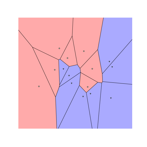
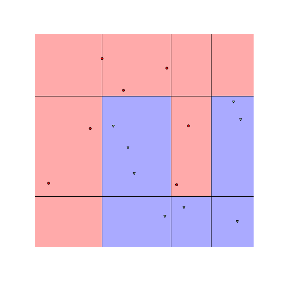
To understand how RBA works, let us look at the figures above. The figures above show the decision boundaries of $1$-NN and decision tree on a toy dataset. We see that the feature space is divided into many regions, where examples in the same region have the same prediction (meaning we can assign a label to each region). These regions are convex for nearest neighbors and tree-based classifiers.
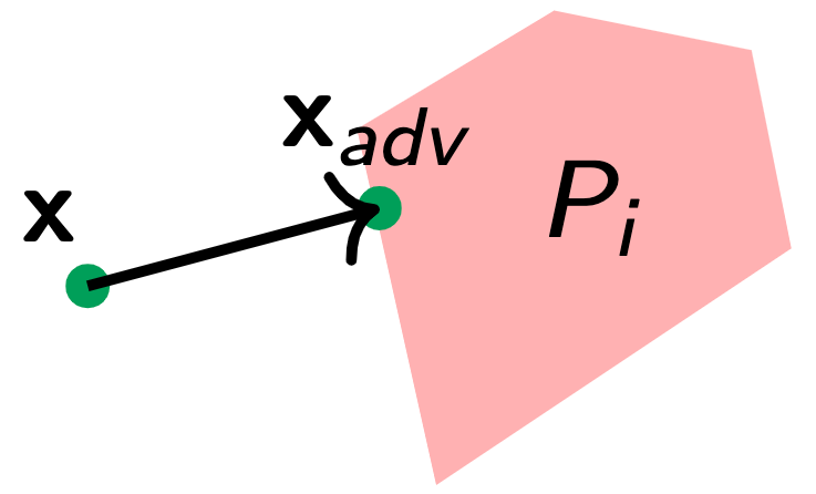
Suppose the example we want to attack is $\mathbf{x}$ and $y$ is its label. RBA works as follows. Suppose we could find the region $P_i$ that is the closest to $\mathbf{x}$ and its label is not $y$. Then, the closest example in $P_i$ to $\mathbf{x}$ would be the optimal adversarial example. RBA finds the closest region $P_i$ by iterating through each region that is labeled differently from $y$. More formally, given a set of regions and its corresponding label $(P_i, y_i)$, the RBA solves the following optimization problem:
The $\textcolor{red}{\text{outer $min$}}$ can be solved by iterating through all regions. The $\textcolor{ForestGreen}{\text{inner $min$}}$ can be solved with standard linear programming when $p=1$ and $\infty$ and quadratic programming when $p=2$. When this optimization problem is solved exactly, we call it RBA-Exact.
Interestingly, concurrent works [1, 2, 3, 4] have also shown that the decision regions of ReLU networks are also decomposable into convex regions and developed attacks based on this property.
Speeding up RBA. Different non-parametric methods divide the feature space into different numbers of regions. When attacking $k$-NN, there would be $O(\binom{N}{k})$ regions, where $N$ is the number of training examples. When attacking RF, there is an exponential number of regions with growing number of trees. It is computationally infeasible to solve RBA-Exact when the number of regions is large.
We develop an approximate version of RBA (RBA-Approx.) to speed up the process and make our algorithm applicable to real datasets. We relax the $\textcolor{red}{\text{outer $min$}}$ by iterating over only a fixed number of regions based on the following two criteria. First, a region has to have at least one training example in it to be considered. Second, if $\mathbf{x}_i$ is the training example in the region $P_i$, then the regions with smaller $\|\mathbf{x}_i - \mathbf{x}\|_p$ are considered first until we exceed the number of regions we want to search. We found that empirically using these two criteria to search $50$ regions can find adversarial examples very close to the target example.
Empirical Results
We empirically evaluate the performance of our attack (RBA) and defense (AP) algorithms.
Evaluation criteria for attacks. We use the distance between an input $\mathbf{x}$ and its generated adversarial example $\mathbf{x}_{adv}$ to evaluate the performance of the attack algorithm. We call this criterion empirical robustness (ER) The lower ER is, the better the attack algorithm is. We calculate the average ER over correctly predicted test examples.
Evaluation criteria for defenses. To evaluate the performance of a defense algorithm, we use the ratio of the distance between an input $\mathbf{x}$ and its closest adversarial example being found before and after the defense algorithm is applied. We call this criterion defense score ($\text{defscore}$). More formally,
We calculate the average defscore over the correctly predicted test examples. A larger defscore means that the attack algorithm needs a larger perturbation to change the label. Thus, the more effective the defense algorithm is. If the defscore is larger than one, then the defense is effectively making the classifier more robust.
We consider the following non-parametric classifiers: $1$ nearest neighbor ($1$-NN), $3$ nearest neighbor ($3$-NN), and random forest (RF).
Attacks. To evaluate RBA, we compare with other attack algorithms for non-parametric methods. Direct attack is designed to attack nearest neighbor classifiers. Black box attack (BBox) is another algorithm that applies to many non-parametric methods. However, as a black-box attack, it does not use the internal structure of the classifier. It appears that BBox is the state-of-the-art algorithm for attacking non-parametric methods.
| $1$-NN | $3$-NN | RF | |||||||
|---|---|---|---|---|---|---|---|---|---|
| Dataset | Direct | BBox | RBA Exact | RBA Approx. | Direct | BBox | RBA Approx. | BBox | RBA Approx. |
| cancer | .223 | .364 | .137 | .137 | .329 | .376 | .204 | .451 | .383 |
| covtype | .130 | .130 | .066 | .067 | .200 | .259 | .108 | .233 | .214 |
| diabetes | .074 | .112 | .035 | .035 | .130 | .143 | .078 | .181 | .184 |
| halfmoon | .070 | .070 | .058 | .058 | .105 | .132 | .096 | .182 | .149 |
From the result, we see that the RBA algorithm is able to perform well across many non-parametric methods and datasets (for results on more datasets and classifiers, please refer our paper). For $1$-NN, RBA-Exact performed the best as expected since its optimal. For $3$-NN and RF, RBA-Approx. also performed the best among the baselines.
Defenses. For baseline, we consider WJC for the defense of $1$-NN and robust splitting (RS) for tree-based classifiers. Another baseline is the adversarial training (AT), which has a lot of success in parametric classifiers. We use RBA-Exact to attack $1$-NN and RBA-Approx to attack $3$-NN and RF for the calculation of defscore.
| $1$-NN | $3$-NN | RF | ||||||
|---|---|---|---|---|---|---|---|---|
| Dataset | AT | WJC | AP | AT | AP | AT | RS | AP |
| cancer | 0.82 | 1.05 | 1.41 | 1.06 | 1.39 | 0.87 | 1.54 | 1.26 |
| covtype | 0.61 | 4.38 | 4.38 | 0.88 | 3.31 | 1.02 | 1.01 | 2.13 |
| diabetes | 0.83 | 4.69 | 4.69 | 0.87 | 2.97 | 1.19 | 1.25 | 2.22 |
| halfmoon | 1.05 | 2.00 | 2.78 | 0.93 | 1.92 | 1.04 | 1.01 | 1.82 |
From the table, we see that AP performs well across different classifiers. AP always generates above $1.0$ defscore, which means the classifier becomes more robust after the defense. This shows that AP is applicable to many non-parametric classifiers as oppose to WJC and RS, which are classifier-specific defenses. AT performs poorly for non-parametric classifiers (this is aligned with previous findings.) This result demonstrates that AP can serve as a good baseline for a new non-parametric classifier.
Conclusion
In this blog post, we consider adversarial examples for non-parametric classifiers and presented generic defenses and attacks. The defense algorithm – adversarial pruning – bridges the gap between $r$-separated and non-$r$-separated data by removing the minimum number of examples to make the data well-separated. Adversarial pruning can be interpreted as a finite sample approximation to the $r$-optimal classifier, which is the most robust classifier under attack radius $r$. The attack algorithm – region-based attack – finds the closest adversarial example and achieves the optimal attack. On the experiment side, we show that both these algorithms are able to perform well across multiple non-parametric classifiers. They can be good candidates for baseline evaluation of robustness for newly designed non-parametric classifiers.
More Details
See our paper on arxiv or our repository.